

Application and Optimisation of the Spatial Phase Shifting ...
Application and Optimisation of the Spatial Phase Shifting ...
Application and Optimisation of the Spatial Phase Shifting ...

You also want an ePaper? Increase the reach of your titles
YUMPU automatically turns print PDFs into web optimized ePapers that Google loves.
3.2 <strong>Phase</strong>-shifting ESPI 59<br />
ϕ<br />
ϕ<br />
O,<br />
i<br />
O,<br />
f<br />
I3i<br />
( x, y) − I1i<br />
( x, y)<br />
( x, y) mod 2π<br />
= arctan<br />
I ( x, y) − I ( x, y)<br />
0i<br />
2i<br />
I3 f ( x, y) − I1f<br />
( x, y)<br />
( x, y) mod 2π<br />
= arctan<br />
I ( x, y) − I ( x, y)<br />
0 f 2 f<br />
, (3.22)<br />
<strong>and</strong> <strong>the</strong>n determine <strong>the</strong> phase change<br />
( O, f<br />
O,<br />
i )<br />
∆ϕ ( x, y) mod 2 π = ϕ ( x, y) mod 2π − ϕ ( x, y)<br />
mod 2π mod 2π<br />
. (3.23)<br />
Admittedly, this requires more information than <strong>the</strong> phase-<strong>of</strong>-difference approach – 8 images with (3.16),<br />
<strong>and</strong> 6 with (3.17) –, but eliminates all <strong>the</strong> problems brought about by <strong>the</strong> ambiguity <strong>of</strong> intensity<br />
differences. Also, <strong>the</strong> pixels are truly regarded as independent entities, which accounts appropriately for<br />
<strong>the</strong> speckle nature <strong>of</strong> <strong>the</strong> wavefront to determine. In this case, <strong>the</strong> phase calculation reproduces <strong>the</strong><br />
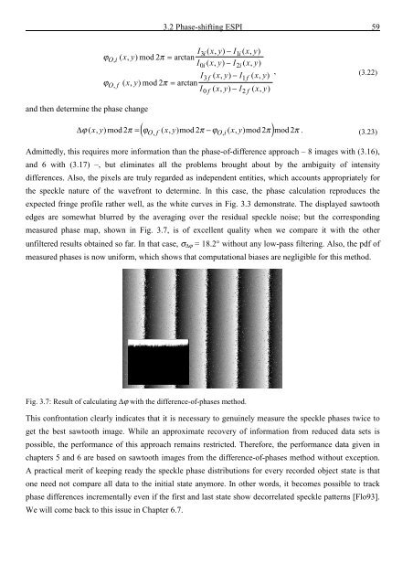
expected fringe pr<strong>of</strong>ile ra<strong>the</strong>r well, as <strong>the</strong> white curves in Fig. 3.3 demonstrate. The displayed sawtooth<br />
edges are somewhat blurred by <strong>the</strong> averaging over <strong>the</strong> residual speckle noise; but <strong>the</strong> corresponding<br />
measured phase map, shown in Fig. 3.7, is <strong>of</strong> excellent quality when we compare it with <strong>the</strong> o<strong>the</strong>r<br />
unfiltered results obtained so far. In that case, σ ∆ϕ = 18.2° without any low-pass filtering. Also, <strong>the</strong> pdf <strong>of</strong><br />
measured phases is now uniform, which shows that computational biases are negligible for this method.<br />
Fig. 3.7: Result <strong>of</strong> calculating ∆ϕ with <strong>the</strong> difference-<strong>of</strong>-phases method.<br />
This confrontation clearly indicates that it is necessary to genuinely measure <strong>the</strong> speckle phases twice to<br />
get <strong>the</strong> best sawtooth image. While an approximate recovery <strong>of</strong> information from reduced data sets is<br />
possible, <strong>the</strong> performance <strong>of</strong> this approach remains restricted. Therefore, <strong>the</strong> performance data given in<br />
chapters 5 <strong>and</strong> 6 are based on sawtooth images from <strong>the</strong> difference-<strong>of</strong>-phases method without exception.<br />
A practical merit <strong>of</strong> keeping ready <strong>the</strong> speckle phase distributions for every recorded object state is that<br />
one need not compare all data to <strong>the</strong> initial state anymore. In o<strong>the</strong>r words, it becomes possible to track<br />
phase differences incrementally even if <strong>the</strong> first <strong>and</strong> last state show decorrelated speckle patterns [Flo93].<br />
We will come back to this issue in Chapter 6.7.


![Skript zur Vorlesung [PDF; 40,0MB ;25.07.2005] - Institut für Physik](https://img.yumpu.com/28425341/1/184x260/skript-zur-vorlesung-pdf-400mb-25072005-institut-fa-1-4-r-physik.jpg?quality=85)


