Application and Optimisation of the Spatial Phase Shifting ...

142 Improvements on SPS
0.12
σ d /λ
0.10
0.08
0.06
0.04
0.02
0.00
0 0
20 20
50 50
100 100
1 10 B 100
N x
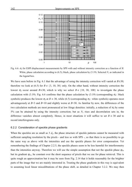
Fig. 6.6: σ d for ESPI displacement measurements by SPS with and without intensity correction as a function of B.
White, phase calculation according to (6.5); black, phase calculation by (3.19). Selected N x as indicated in
the legend box.
We have seen before in Fig. 6.1 that the advantage of using the intensity correction will vanish at B30;
therefore we look at (6.5) for B ∈ {3, 10, 30} only. On the other hand, without intensity correction the
lowest σ d occur around B30, which is why we select B ∈ {10, 30, 100} to investigate the phase
calculation with (3.19). Fig. 6.6 confirms that the phase calculation by (3.19) (corresponding σ d : black
symbols) produces the lowest σ d at B 30, while (6.5) (corresponding σ d : white symbols) operates most
advantageously at B=3 and B=10 and slightly worse at B=30. As familiar by now, the differences of the
two calculation methods are most pronounced at low fringe densities: initially, a reduction of σ d by some
5% can be attained by using the intensity correction; but as N x rises and decorrelation sets in, the
difference vanishes almost completely. Hence, in most situations it will suffice to set B 30 and to
record interferograms only.
6.2.2 Consideration of speckle phase gradients
When the speckles are as small as 3 d p , the phase structure of speckle patterns cannot be measured with
sufficient sampling resolution by the pixels - and less so with SPS -, so that there is no possibility to go
the same way as above with the intensities and use the speckle phases for error compensation. Yet
remembering the findings of Chapter 2.2.5, the speckle phases seem to be less harmful for interferometry
than the intensities anyway. Therefore we will use the simple assumption that not the speckle phase ϕ O ,
but its gradient ϕ O,x be constant over the short sequence of pixels that we use for phase retrieval. This is
quite rough an approximation but it may be seen from Fig. 2.14 that it holds reasonably for the brighter
parts of the image that we are mainly interested in. Treating the phase gradients in this way is equivalent
to assuming local linear miscalibrations of the phase shift, as detailed in Chapter 3.2.2. We may then