Application and Optimisation of the Spatial Phase Shifting ...

108 Quantification of displacement-measurement errors
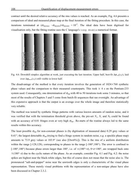
contract until the desired relative accuracy of the rms values is reached. As an example, Fig. 4.6 presents a
comparison of ideal and measured phase map at the final iteration of the fitting procedure. In this case, the
iterations terminated at (σ ∆ϕ,max –σ ∆ϕ,min )/σ ∆ϕ,min = 10 -5 . The ideal data have been digitised for
visualisation only, but the fitting routine uses the C language's long double numerical format.
Fig. 4.6: Downhill simplex algorithm at work, just executing the last iteration. Upper half, best-fit ∆ϕ ref(x,y), laid
over ∆ϕ meas (x,y) still visible in lower half.
The disadvantage of the method is that every iteration involves the generation of 1024768 synthetic
phase values and the comparison to their measured counterparts. This took 4 s on the Pentium-233
system used. Consequently, one determination of σ ∆ϕ with 40 to 50 iterations took some 3 minutes, so that
most of the results of Chapters 5 and 5 come from batch-fit sequences that ran overnight. An advantage of
this expensive approach is that the output is an average over the whole image and therefore statistically
very reliable.
The method was tested by synthetic fringe patterns with various known amounts of random noise, and it
was verified that with the termination threshold given above, the pre-set N x , N y and N 0 could be found
with an accuracy of 0.01 fringes even at very high σ ∆ϕ . Re-starts of the routine always led to the same
results within this accuracy.
The least possible σ ∆ϕ for non-constant phases is (by digitisation of measured data) 0.29 grey values or
0.41°; the largest detectable σ ∆ϕ (trying to find a fringe system in random noise, e.g. a speckle phase map)
amounts to 73.9 grey values or 103.9° (see also [Own91c]). This is the rms of a uniform distribution
within the range [-128,128), corresponding to phases in the range [-180°,180°). The error is confined to
[-180°,180°) because phase errors larger than 180°, i.e. of (180°+ε), 0