

Application and Optimisation of the Spatial Phase Shifting ...
Application and Optimisation of the Spatial Phase Shifting ...
Application and Optimisation of the Spatial Phase Shifting ...

Create successful ePaper yourself
Turn your PDF publications into a flip-book with our unique Google optimized e-Paper software.
2.3 Second-order speckle statistics 39<br />
p (I 1 ,I 2 )<br />
0.4<br />
0.3<br />
0.2<br />
0<br />
0.1<br />
0.25<br />
0.5<br />
µ A 0.75<br />
0.95<br />
1<br />
I 2 /I 1<br />
2<br />
0<br />
3<br />
0<br />
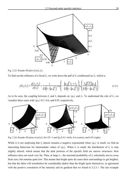
Fig. 2.23: Pseudo-3D plot <strong>of</strong> p(I 1 ,I 2 ).<br />
To find out <strong>the</strong> influence <strong>of</strong> a fixed I 1 , we write down <strong>the</strong> pdf <strong>of</strong> I 2 conditioned on I 1 , which is<br />
( | I )<br />
p I<br />
2 1<br />
( , I )<br />
p I1 2<br />
= =<br />
p I<br />
1<br />
⎛<br />
⎜<br />
µ<br />
2<br />
A I1 + I2<br />
exp<br />
I<br />
( ) 2<br />
⎜−<br />
2<br />
⎟ 0⎜<br />
2<br />
1 I ( 1−<br />
µ A ) ⎜<br />
⎝<br />
I ( 1−<br />
µ A ) ⎟ ⎜<br />
⎠ ⎝<br />
I ( 1−<br />
µ A )<br />
⎞<br />
⎟<br />
⎛<br />
⎜<br />
2<br />
I I<br />
1 2<br />
µ<br />
A<br />
⎞<br />
⎟<br />
⎟ . (2.51)<br />
⎟<br />
⎠<br />
As to be seen, <strong>the</strong> coupling between I 2 <strong>and</strong> I 1 depends on Fµ Α F <strong>and</strong> I 1 . To underst<strong>and</strong> <strong>the</strong> role <strong>of</strong> I 1 , we<br />
visualise three cases with Fµ Α F=0.1, 0.6, <strong>and</strong> 0.95, respectively.<br />
0<br />
0.5<br />
0<br />
1<br />
2<br />
0<br />
I 3 1<br />
0<br />
1<br />
3<br />
2 I 2<br />
1<br />
p (I 2 |I 1 )<br />
p (I 2 |I 1 )<br />
1.5<br />
1<br />
0.5<br />
0<br />
1<br />
2<br />
0<br />
I 3 1<br />
0<br />
1<br />
3<br />
2 I 2<br />
1<br />
2<br />
10<br />
p (I 2 |I 1 )<br />
0<br />
3 1<br />
0<br />
3<br />
2<br />
I 1 I 2<br />
5<br />
Fig. 2.24: Pseudo-3D plots <strong>of</strong> p(I 2 |I 1 ) for ¡I¢=1 <strong>and</strong> µ Α =0.1 (left), 0.6 (centre), <strong>and</strong> 0.95 (right).<br />
While it is not surprising that I 2 almost remains a negative exponential when Fµ Α F is small, we find an<br />
interesting behaviour for intermediate values <strong>of</strong> Fµ Α F. When I 1 is small, <strong>the</strong> distribution <strong>of</strong> I 2 is only<br />
slightly altered, which means that <strong>the</strong> dark portions <strong>of</strong> <strong>the</strong> speckle field are narrow structures: <strong>the</strong>ir<br />
influence does not reach very far. Then, at large I 1 , <strong>the</strong> maximal probability <strong>of</strong> I 2 reluctantly moves away<br />
from zero, but remains quite low. This means that bright spots do cause <strong>the</strong>ir surroundings to get brighter,<br />
but that <strong>the</strong> latter will none<strong>the</strong>less be considerably darker than <strong>the</strong> bright spots <strong>the</strong>mselves, in agreement<br />
with <strong>the</strong> positive correlation <strong>of</strong> <strong>the</strong> intensity <strong>and</strong> its gradient that we found in 2.2.3.1. The last example


![Skript zur Vorlesung [PDF; 40,0MB ;25.07.2005] - Institut für Physik](https://img.yumpu.com/28425341/1/184x260/skript-zur-vorlesung-pdf-400mb-25072005-institut-fa-1-4-r-physik.jpg?quality=85)


