

Application and Optimisation of the Spatial Phase Shifting ...
Application and Optimisation of the Spatial Phase Shifting ...
Application and Optimisation of the Spatial Phase Shifting ...

You also want an ePaper? Increase the reach of your titles
YUMPU automatically turns print PDFs into web optimized ePapers that Google loves.
128 Comparison <strong>of</strong> noise in phase maps from TPS <strong>and</strong> SPS<br />
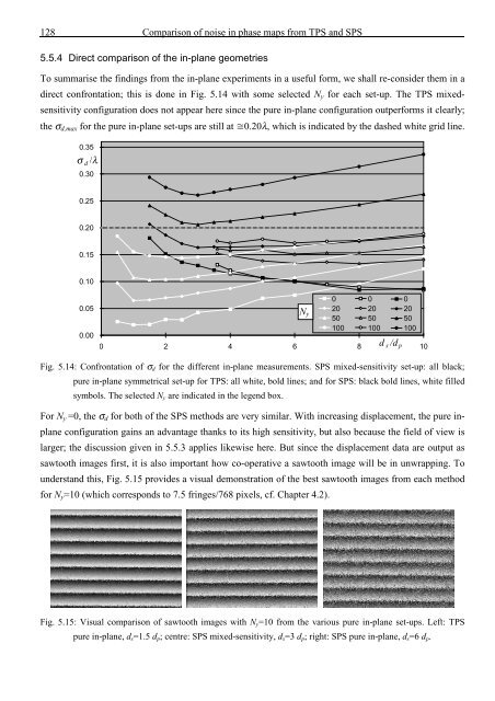
5.5.4 Direct comparison <strong>of</strong> <strong>the</strong> in-plane geometries<br />
To summarise <strong>the</strong> findings from <strong>the</strong> in-plane experiments in a useful form, we shall re-consider <strong>the</strong>m in a<br />
direct confrontation; this is done in Fig. 5.14 with some selected N y for each set-up. The TPS mixedsensitivity<br />
configuration does not appear here since <strong>the</strong> pure in-plane configuration outperforms it clearly;<br />
<strong>the</strong> σ d,max for <strong>the</strong> pure in-plane set-ups are still at 0.20λ, which is indicated by <strong>the</strong> dashed white grid line.<br />
0.35<br />
σ d /λ<br />
0.30<br />
0.25<br />
0.20<br />
0.15<br />
0.10<br />
0.05<br />
0.00<br />
0 0 0<br />
20 20 20<br />
50 50 50<br />
100 100 100<br />
0 2 4 6 8<br />
d s /d p 10<br />
N y<br />
Fig. 5.14: Confrontation <strong>of</strong> σ d for <strong>the</strong> different in-plane measurements. SPS mixed-sensitivity set-up: all black;<br />
pure in-plane symmetrical set-up for TPS: all white, bold lines; <strong>and</strong> for SPS: black bold lines, white filled<br />
symbols. The selected N y are indicated in <strong>the</strong> legend box.<br />
For N y =0, <strong>the</strong> σ d for both <strong>of</strong> <strong>the</strong> SPS methods are very similar. With increasing displacement, <strong>the</strong> pure inplane<br />
configuration gains an advantage thanks to its high sensitivity, but also because <strong>the</strong> field <strong>of</strong> view is<br />
larger; <strong>the</strong> discussion given in 5.5.3 applies likewise here. But since <strong>the</strong> displacement data are output as<br />
sawtooth images first, it is also important how co-operative a sawtooth image will be in unwrapping. To<br />
underst<strong>and</strong> this, Fig. 5.15 provides a visual demonstration <strong>of</strong> <strong>the</strong> best sawtooth images from each method<br />
for N y =10 (which corresponds to 7.5 fringes/768 pixels, cf. Chapter 4.2).<br />
Fig. 5.15: Visual comparison <strong>of</strong> sawtooth images with N y =10 from <strong>the</strong> various pure in-plane set-ups. Left: TPS<br />
pure in-plane, d s =1.5 d p ; centre: SPS mixed-sensitivity, d s =3 d p ; right: SPS pure in-plane, d s =6 d p .


![Skript zur Vorlesung [PDF; 40,0MB ;25.07.2005] - Institut für Physik](https://img.yumpu.com/28425341/1/184x260/skript-zur-vorlesung-pdf-400mb-25072005-institut-fa-1-4-r-physik.jpg?quality=85)


