Application and Optimisation of the Spatial Phase Shifting ...

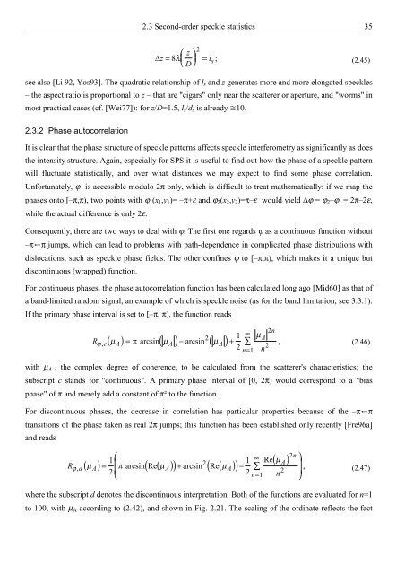
2.3 Second-order speckle statistics 35
2
⎛ z ⎞
∆z = 8λ ⎜ ⎟ = l
⎝ D⎠
s ; (2.45)
see also [Li 92, Yos93]. The quadratic relationship of l s and z generates more and more elongated speckles
– the aspect ratio is proportional to z – that are "cigars" only near the scatterer or aperture, and "worms" in
most practical cases (cf. [Wei77]): for z/D=1.5, l s /d s is already 10.
2.3.2 Phase autocorrelation
It is clear that the phase structure of speckle patterns affects speckle interferometry as significantly as does
the intensity structure. Again, especially for SPS it is useful to find out how the phase of a speckle pattern
will fluctuate statistically, and over what distances we may expect to find some phase correlation.
Unfortunately, ϕ is accessible modulo 2π only, which is difficult to treat mathematically: if we map the
phases onto [–π,π), two points with ϕ 1 (x 1 ,y 1 )= –π+ε and ϕ 2 (x 2 ,y 2 )=π–ε would yield ∆ϕ = ϕ 2 –ϕ 1 = 2π–2ε,
while the actual difference is only 2ε.
Consequently, there are two ways to deal with ϕ. The first one regards ϕ as a continuous function without
–ππ jumps, which can lead to problems with path-dependence in complicated phase distributions with
dislocations, such as speckle phase fields. The other confines ϕ to [–π,π), which makes it a unique but
discontinuous (wrapped) function.
For continuous phases, the phase autocorrelation function has been calculated long ago [Mid60] as that of
a band-limited random signal, an example of which is speckle noise (as for the band limitation, see 3.3.1).
If the primary phase interval is set to [–π, π), the function reads
2
( ) π ( ) ( )
Rϕ , c µ A = arcsin µ A − arcsin µ A +
1
2
∞
∑
n=
1
µ
2n
A
2
n
, (2.46)
with µ A , the complex degree of coherence, to be calculated from the scatterer's characteristics; the
subscript c stands for "continuous". A primary phase interval of [0, 2π) would correspond to a "bias
phase" of π and merely add a constant of π² to the function.
For discontinuous phases, the decrease in correlation has particular properties because of the –ππ
transitions of the phase taken as real 2π jumps; this function has been established only recently [Fre96a]
and reads
1
⎛
Rϕ , d ( µ A) = ⎜
2 1
π arcsin( Re( µ A)
) + arcsin ( Re( µ A)
) −
2 ⎜
⎝
2
∞
∑
n=
1
Re
( µ )
n
A
2
2n
⎞
⎟ ,
⎟
(2.47)
⎠
where the subscript d denotes the discontinuous interpretation. Both of the functions are evaluated for n=1
to 100, with µ A according to (2.42), and shown in Fig. 2.21. The scaling of the ordinate reflects the fact