Application and Optimisation of the Spatial Phase Shifting ...

6.5 Fourier transform method of phase determination 155
( , ν )
Bδ νx y
( − 0 − 0 )
B ~ *
o νx ν x , ν y ν y
log P/a.u.
v N
v N
v y
0 0 v x
~
O( ν x , ν y )
-v N
~ 2
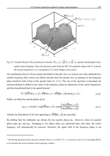
Fig. 6.17: Pseudo-3D plot of the spectral power density P( ν , ν ) = I ( ν , ν ) in a speckle interferogram with a
x y x y
spatial carrier frequency. Since the spectrum comes from the DFT of a quadratic image with N N pixels,
the Nyqvist frequencies ¡ν N correspond to N/2 carrier fringes on the sensor.
All contributions from (6.18) are clearly discernible in the plot. Now we enclose one of the sidebands by a
suitable frequency filter whose size follows directly from the speckle size; its diameter in the frequency
plane should be half of that of the speckle halo (cf. 3.3.1). The rest of the spectrum is discarded; the
selected sideband is shifted to the centre of the frequency plane by subtraction of the carrier frequencies,
and then transformed back to the spatial domain: *
( )
FT -1 B ~ r ~( o ν , ν ) = B r o ( x , y ) = B r o ( x , y ) exp( i ϕ ( x , y )) ; (6.20)
finally, we obtain the speckle phases ϕ O by
ϕ
x y O
⎛ ( )
O x y π ( B x y B x y
( , ) arg ( , ))
arctan Im ro
mod2 = ro =
( , )
⎜
⎝ Re( Bro
( x, y)
)
whereby the fluctuations of M I , here appearing as Br o ( x, y)
, are cancelled.
⎞
⎟
, (6.21)
⎠
By shifting back the sidebands, one obtains the true speckle phases ϕ O . However, when two speckle
phase maps ϕ O,i and ϕ O,f , belonging to two object states, are subtracted from each other, the carrier
frequency will automatically be removed. Therefore, the signal shift in the frequency plane is not
* The filtering operations destroy the point symmetry about ν x =ν y =0 that I ~ ( νx , ν y ) possesses as the FT of a real signal [Bra87,
p.14]; therefore the inverse transform will be genuinely complex.