Application and Optimisation of the Spatial Phase Shifting ...

96 Electronic or Digital Speckle Pattern Interferometry
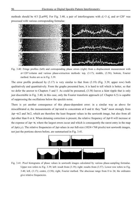
methods should be 4/3 [Lar99]. For Fig. 3.40, a pair of interferograms with d s =3 d p and α=120° was
processed with various corresponding formulae.
Fig. 3.40: Fringe profiles (left) and corresponding phase errors (right) from a displacement measurement with
α=120°/column and various phase-extraction methods: top, (3.17); middle, (3.58); bottom, Fourier
method. Scales are as in Fig. 3.39.
The error profile produced by (3.17) is very similar to that from (3.19) (Fig. 3.39, upper row) both
qualitatively and quantitatively. From the graphs presented here, it is hard to tell which is better, so that
we defer the answer to Chapters 5 and 5. As could be presumed, (3.58) leaves a faint ripple that is only
just discernible in Fig. 3.40; in this case, only the Fourier transform approach (cf. Chapter 6.5) is capable
of suppressing the oscillations below the speckle noise.
There is yet another consequence of this phase-dependent error: in a similar way as above for
miscalibrated α, the measurements of ∆ϕ tend to concentrate at 0 and π: they "leak" most strongly from
∆ϕ =π/2 and 3π/2, which are therefore the least frequent values in the sawtooth image, but also from all
∆ϕ other than 0 or π. When detuning correction is present, the relative frequency of ∆ϕ=0 will increase at
the expense of ∆ϕ =π, where the largest errors occur and which is consequently the rarest entry in the map
of ∆ϕ (x,y). The relative frequencies of ∆ϕ values in our full-size (1024768 pixels) test sawtooth images,
not just the portions shown before, are summarised in Fig. 3.41.
Fig. 3.41: Pixel histograms of phase values in sawtooth images calculated by various phase-sampling formulae.
Upper row refers to Fig. 3.39; left: result from (3.19); right: results from (3.57). Lower row refers to Fig.
3.40; left, (3.17); centre, (3.58); right, Fourier method. The abscissae range from 0 to 2π; the ordinates
give relative frequencies.