

Application and Optimisation of the Spatial Phase Shifting ...
Application and Optimisation of the Spatial Phase Shifting ...
Application and Optimisation of the Spatial Phase Shifting ...

You also want an ePaper? Increase the reach of your titles
YUMPU automatically turns print PDFs into web optimized ePapers that Google loves.
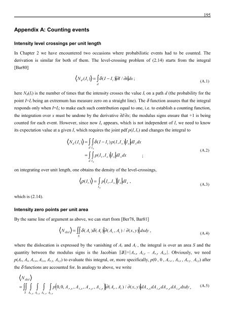
195<br />
Appendix A: Counting events<br />
Intensity level crossings per unit length<br />
In Chapter 2 we have encountered two occasions where probabilistic events had to be counted. The<br />
derivation is similar for both <strong>of</strong> <strong>the</strong>m. The level-crossing problem <strong>of</strong> (2.14) starts from <strong>the</strong> integral<br />
[Bar80]<br />
Nd ( It ) = ∫ δ ( I − It<br />
) ∂ I / ∂ x dx ; (A.1)<br />
d<br />
here N d (I t ) is <strong>the</strong> number <strong>of</strong> times that <strong>the</strong> intensity crosses <strong>the</strong> value I t on a path d (<strong>the</strong> probability for <strong>the</strong><br />
point I=I t being an extremum has measure zero on a straight line). The δ function assures that <strong>the</strong> integral<br />
responds only when I=I t ; to make each such contribution equal to one, i.e. to establish a counting function,<br />
<strong>the</strong> integration over x must be undone by <strong>the</strong> derivative ∂I/∂x; <strong>the</strong> modulus signs ensure that +1 is being<br />
counted for each event. However, since now I x appears, which is not independent <strong>of</strong> I, we need to know<br />
its expectation value at a given I, which requires <strong>the</strong> joint pdf p(I, I x ) <strong>and</strong> changes <strong>the</strong> integral to<br />
N ( I ) = δ ( I − I ) p( I, I ) I dI dx<br />
d t t x x x<br />
d Ix<br />
=<br />
∫ ∫<br />
∫ ∫<br />
d Ix<br />
p( I , I ) I dI dx<br />
t x x x<br />
on integrating over unit length, one obtains <strong>the</strong> density <strong>of</strong> <strong>the</strong> level-crossings,<br />
( )<br />
ρ( I ) = ∫ p I , I I dI ,<br />
t t x x x<br />
I x<br />
;<br />
(A.2)<br />
(A.3)<br />
which is (2.14).<br />
Intensity zero points per unit area<br />
By <strong>the</strong> same line <strong>of</strong> argument as above, we can start from [Ber78, Bar81]<br />
N ( A ) ( A ) ( A , A ) / ( x , y ) dxdy , (A.4)<br />
= ∫∫ δ δ ∂ ∂<br />
disl r i r i<br />
S<br />
where <strong>the</strong> dislocation is expressed by <strong>the</strong> vanishing <strong>of</strong> A r <strong>and</strong> A i , <strong>the</strong> integral is over an area S <strong>and</strong> <strong>the</strong><br />
quantity between <strong>the</strong> modulus signs is <strong>the</strong> Jacobian GJG=FA r,x A i,y – A r,y A i,x F. Obviously, we need<br />
p(A r , A i , A r,x , A i,x , A r,y, A i,y ) to evaluate this integral, or, more specifically, p(0 , 0 , A r,x , A i,x , A r,y , A i,y ) after<br />
<strong>the</strong> δ functions are accounted for. In analogy to above, we write<br />
N<br />
disl<br />
( )<br />
= ∫∫ ∫ ∫ ∫ ∫ p 0, 0, A r, x , A i, x , A r, y , A i, y ∂( Ar , Ai ) / ∂ ( x, y)<br />
dA r, xdA i, xdA r, ydA i,<br />
ydxdy<br />
, (A.5)<br />
S Ar , x Ai , x Ar , y Ai , x


![Skript zur Vorlesung [PDF; 40,0MB ;25.07.2005] - Institut für Physik](https://img.yumpu.com/28425341/1/184x260/skript-zur-vorlesung-pdf-400mb-25072005-institut-fa-1-4-r-physik.jpg?quality=85)


