Application and Optimisation of the Spatial Phase Shifting ...

34 Statistical Properties of Speckle Patterns
function, which demonstrates that the speckle shape is closely related to the aperture´s point spread
function. It assumes its first zero at
∆x
λ z
+ ∆y
≅ 122 . =
D
2 2
d s
,
(2.43)
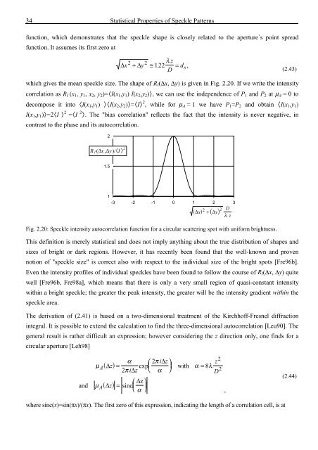
which gives the mean speckle size. The shape of R I (∆x, ∆y) is given in Fig. 2.20. If we write the intensity
correlation as R I (x 1 , y 1 , x 2 , y 2 )=I(x 1 ,y 1 ) I(x 2 ,y 2 ), we can use the independence of P 1 and P 2 at µ A = 0 to
decompose it into I(x 1 ,y 1 ) I(x 2 ,y 2 )=I 2 , while for µ A = 1 we have P 1 =P 2 and obtain I(x 1 ,y 1 )
I(x 1 ,y 1 )=2I 2 =I 2 . The "bias correlation" reflects the fact that the intensity is never negative, in
contrast to the phase and its autocorrelation.
2
R I (∆x ,∆y )/ I ¡ 2 ( ) ( )
1.5
1
-3 -2 -1 0 1 2 3
∆
2 2 D
x + ∆y
λ z
Fig. 2.20: Speckle intensity autocorrelation function for a circular scattering spot with uniform brightness.
This definition is merely statistical and does not imply anything about the true distribution of shapes and
sizes of bright or dark regions. However, it has recently been found that the well-known and proven
notion of "speckle size" is correct also with respect to the individual size of the bright spots [Fre96b].
Even the intensity profiles of individual speckles have been found to follow the course of R I (∆x, ∆y) quite
well [Fre96b, Fre98a], which means that there is only a very small region of quasi-constant intensity
within a bright speckle; the greater the peak intensity, the greater will be the intensity gradient within the
speckle area.
The derivation of (2.41) is based on a two-dimensional treatment of the Kirchhoff-Fresnel diffraction
integral. It is possible to extend the calculation to find the three-dimensional autocorrelation [Leu90]. The
general result is rather difficult an expression; however considering the z direction only, one finds for a
circular aperture [Leh98]
and
α ⎛ 2π
i∆z⎞
z
µ A( ∆z)
= exp⎜
⎟ with α = 8λ
2π
i∆z
⎝ α ⎠
D
⎛ ∆z⎞
µ A( ∆z)
= sinc⎜
⎟
⎝ α ⎠
2
2
,
(2.44)
where sinc(x)=sin(πx)/(πx). The first zero of this expression, indicating the length of a correlation cell, is at