

Application and Optimisation of the Spatial Phase Shifting ...
Application and Optimisation of the Spatial Phase Shifting ...
Application and Optimisation of the Spatial Phase Shifting ...

You also want an ePaper? Increase the reach of your titles
YUMPU automatically turns print PDFs into web optimized ePapers that Google loves.
148 Improvements on SPS<br />
To use <strong>the</strong> intensity correction, we re-define our auxiliary quantities, <strong>the</strong> K n :<br />
( tan ϕ )<br />
O<br />
( tan ϕ )<br />
O<br />
1<br />
2<br />
=<br />
=<br />
O3 ( D4 − D2<br />
)<br />
O ( D − D ) − O ( D − D ) : =<br />
4 2 3 2 3 4<br />
O3 ( D6 − D1<br />
)<br />
O ( D D ) O ( D D ) : =<br />
− − − K<br />
6 1 3 1 3 6<br />
K2<br />
K − K<br />
3 1<br />
K5<br />
− K<br />
6 4<br />
(6.12)<br />
<strong>and</strong> obtain<br />
ϕ<br />
O<br />
mod π = arctan<br />
K2 + K5<br />
− K + K − K + K<br />
1 3 4 6<br />
,<br />
(6.13)<br />
which method <strong>of</strong> averaging is correct for this purpose, since both expressions should yield <strong>the</strong> same<br />
phase. (In this case, <strong>the</strong> inclusion <strong>of</strong> two more quotients from pixels {1, 3, 4} <strong>and</strong> {2, 3, 6} is not<br />
equivalent to a doubling <strong>of</strong> <strong>the</strong> terms; but on doing so, <strong>the</strong> reduction <strong>of</strong> σ d is minimal.) The spectral<br />
transfer properties <strong>of</strong> (6.11) <strong>and</strong> (6.13) are now genuinely two–dimensional, so that we can rewrite (3.73) as<br />
~ ~ ~ ~<br />
( ( , ) ( , ) ) arg ( ( , ) ( , ) )<br />
bsc( νx , νy ) = arg I ~ ( νx , νy ) ⋅ C ~ ( νx , νy ) + I νx νy ⋅ S νx νy − I νx νy ⋅C<br />
νx νy<br />
⎛<br />
~<br />
S ( νx<br />
, νy<br />
) ⎞<br />
= arg<br />
⎜1+<br />
~ ⎝ C ( νx<br />
, νy<br />
) ⎟<br />
⎠<br />
(6.14)<br />
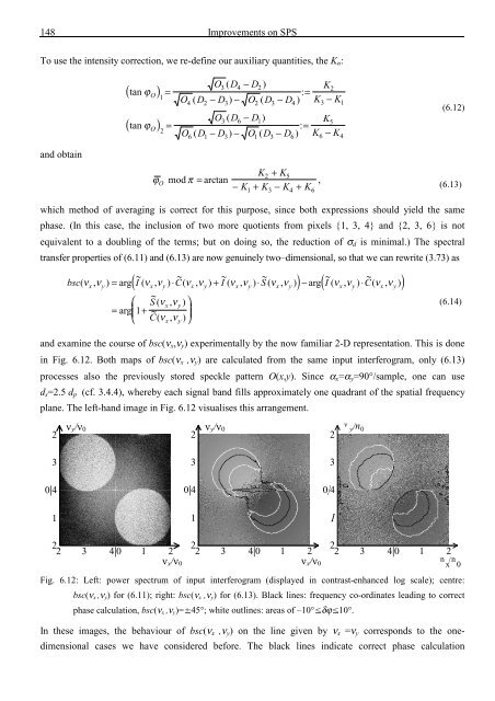
<strong>and</strong> examine <strong>the</strong> course <strong>of</strong> bsc(ν x ,ν y ) experimentally by <strong>the</strong> now familiar 2-D representation. This is done<br />
in Fig. 6.12. Both maps <strong>of</strong> bsc(ν x ,ν y ) are calculated from <strong>the</strong> same input interferogram, only (6.13)<br />
processes also <strong>the</strong> previously stored speckle pattern O(x,y). Since α x =α y =90°/sample, one can use<br />
d s =2.5 d p (cf. 3.4.4), whereby each signal b<strong>and</strong> fills approximately one quadrant <strong>of</strong> <strong>the</strong> spatial frequency<br />
plane. The left-h<strong>and</strong> image in Fig. 6.12 visualises this arrangement.<br />
2<br />
2<br />
2<br />
ν y /n 0<br />
ν y /ν 0<br />
2 3 4|0 1 2<br />
3<br />
3<br />
0|4<br />
1<br />
0|4<br />
1<br />
2<br />
2 3 4|0 1 2<br />
ν x /ν 0<br />
2<br />
ν y /ν 0<br />
2 3 4|0 1 2<br />
3<br />
0|4<br />
1<br />
ν x /ν 0<br />
2<br />
n x<br />
/n 0<br />
Fig. 6.12: Left: power spectrum <strong>of</strong> input interferogram (displayed in contrast-enhanced log scale); centre:<br />
bsc(ν x ,ν y ) for (6.11); right: bsc(ν x ,ν y ) for (6.13). Black lines: frequency co-ordinates leading to correct<br />
phase calculation, bsc(ν x ,ν y )= 45°; white outlines: areas <strong>of</strong> –10°¡δϕ¡10°.<br />
In <strong>the</strong>se images, <strong>the</strong> behaviour <strong>of</strong> bsc(ν x ,ν y ) on <strong>the</strong> line given by ν x =ν y corresponds to <strong>the</strong> onedimensional<br />
cases we have considered before. The black lines indicate correct phase calculation


![Skript zur Vorlesung [PDF; 40,0MB ;25.07.2005] - Institut für Physik](https://img.yumpu.com/28425341/1/184x260/skript-zur-vorlesung-pdf-400mb-25072005-institut-fa-1-4-r-physik.jpg?quality=85)


