Application and Optimisation of the Spatial Phase Shifting ...

197
Appendix B: Real-time phase calculation
To utilise the real-time phase measuring capability that SPS offers, the generation of phase maps must be
accelerated by saving as many processor operations as possible. Particularly the arctangent calls, usually
one for each pixel, lead to a great computational burden that is unnecessary when the input "sine" and
"cosine" terms have a reasonably narrow range of discrete values.
Given the expression
I−1 − I1
ϕOmod 2π
= arctan 3 , 2 I − I − I
(B.1)
0 −1 1
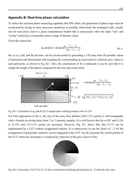
the atan2 call, and the division, can be circumvented by generating a 2-D array from all possible values
of numerator and denominator and assigning the corresponding ϕ O (converted to a discrete grey value) to
each grid point, as shown in Fig. B.1. Also, the construction of M I is indicated; it can be seen that it is
simply the length of the phasor composed by the sine and cosine terms.
(2I 0 –I -1 –I 1 )
– 510 0 510
255
(I -1 –I 1 )
0
j
O
I−1 − I1
= arctan 3 2 I − I − I
0 −1 1
look-up table
2
−1 1
2
0 −1 1
∝ M I = 3 ( I − I ) + ( 2 I − I − I )
– 255
Fig. B.1: Calculation of ϕ O and M I for 3-sample phase shifting formula with α=120°.
For 8-bit digitisation of the I n , the size of the array thus defined (1021511 points) is still manageable
with a formula involving terms from 2 or 3 intensity samples. It is well known that for α=90° and (3.16)
or (3.19), only 511511 points are necessary. However, Fig. B.1 shows that also (3.17) can be
implemented by a LUT without exaggerated expense. It is unnecessary to use the factor of L3 for the
arrangement of grid points; instead it can be integrated in the LUT. Fig. B.2 presents the central portion of
the LUT, where the anisotropy is visualised by reduction of the grey scale to 4 bits.
Fig. B.2: Anisotropy of LUT for (3.17) due to horizontal stretching and inclusion of
3 from the sine term.