Application and Optimisation of the Spatial Phase Shifting ...

24 Statistical Properties of Speckle Patterns
Moreover, the study [Shva95] shows that the major part of the anticorrelation is due to higher intensities
and lower phase gradients. This is mainly due to the relative areas: while intensity minima coincide
almost perfectly with very high phase gradients, they contribute only a very small area fraction to the
speckle field.
As above, we conclude the considerations by confronting them with the experimental findings. Inserting
our C 0 and I into (2.30) and (2.32), we now find F∇IF6.5 grey levels/pixel and F∇ϕF6.6°/pixel.
From the sample image we get measurements of F∇IF6.1 grey levels/pixel and F∇ϕF6.3°/pixel,
where the gradients are approximated by the square root of horizontal plus vertical squared pixel-to-pixeldifferences.
This time, the slight systematic underestimations mentioned above affect both results, since
they are increased by the inclusion of two dimensions; but still the agreement is good. The spatial
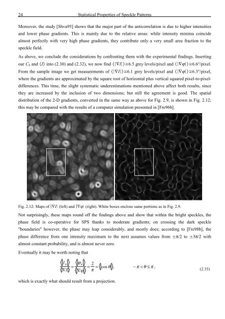
distribution of the 2-D gradients, converted in the same way as above for Fig. 2.9, is shown in Fig. 2.12;
this may be compared with the results of a computer simulation presented in [Fre96b].
Fig. 2.12: Maps of ∇I (left) and ∇ϕ (right). White boxes enclose same portions as in Fig. 2.9.
Not surprisingly, these maps round off the findings above and show that within the bright speckles, the
phase field is co-operative for SPS thanks to moderate gradients; on crossing the dark speckle
"boundaries" however, the phase may leap considerably, and mostly does; according to [Fre98b], the
phase difference from one intensity maximum to the next assumes values from π/2 to 3π/2 with
almost constant probability, and is almost never zero.
Eventually it may be worth noting that
I
x
ϕ
x
∇ I
= ∇ϕ
2
= = cos θ , − π < θ ≤ π ,
π
(2.33)
which is exactly what should result from a projection.