

Application and Optimisation of the Spatial Phase Shifting ...
Application and Optimisation of the Spatial Phase Shifting ...
Application and Optimisation of the Spatial Phase Shifting ...

You also want an ePaper? Increase the reach of your titles
YUMPU automatically turns print PDFs into web optimized ePapers that Google loves.
3.4 <strong>Spatial</strong> phase shifting 93<br />
although such a test is not possible with <strong>the</strong> three-step 90° formulae, <strong>the</strong> findings thus far strongly indicate<br />
a similar behaviour.<br />
In <strong>the</strong> error-compensating formula (3.56), S(n) requires only two samples but C(n) uses four, whilst in<br />
(3.57), both terms include four samples; but also for <strong>the</strong>se methods, <strong>the</strong> performances are virtually<br />
identical. Therefore we will not compare <strong>the</strong>se in detail, but we do investigate <strong>the</strong> performance <strong>of</strong> (3.56)<br />
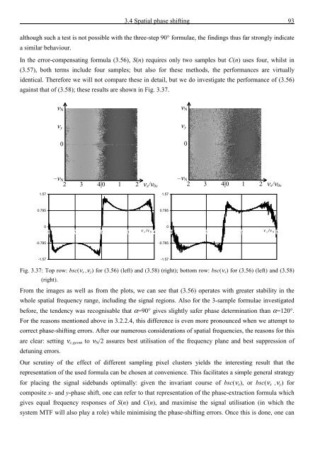
against that <strong>of</strong> (3.58); <strong>the</strong>se results are shown in Fig. 3.37.<br />
ν N<br />
ν N<br />
ν y<br />
0<br />
ν y<br />
0<br />
–ν N –ν N<br />
2 3 4|0 1 2 ν x /ν 0x 2 3 4|0 1 2 ν x /ν 0x<br />
1.57<br />
1.57<br />
0.785<br />
0.785<br />
0<br />
0 1 2 3 4<br />
0<br />
0 1 2 ν x /ν 0 3<br />
-0.785<br />
ν x /ν 0<br />
-0.785<br />
-1.57<br />
-1.57<br />
Fig. 3.37: Top row: bsc(ν x ,ν y ) for (3.56) (left) <strong>and</strong> (3.58) (right); bottom row: bsc(ν x ) for (3.56) (left) <strong>and</strong> (3.58)<br />
(right).<br />
From <strong>the</strong> images as well as from <strong>the</strong> plots, we can see that (3.56) operates with greater stability in <strong>the</strong><br />
whole spatial frequency range, including <strong>the</strong> signal regions. Also for <strong>the</strong> 3-sample formulae investigated<br />
before, <strong>the</strong> tendency was recognisable that α=90° gives slightly safer phase determination than α=120°.<br />
For <strong>the</strong> reasons mentioned above in 3.2.2.4, this difference is even more pronounced when we attempt to<br />
correct phase-shifting errors. After our numerous considerations <strong>of</strong> spatial frequencies, <strong>the</strong> reasons for this<br />
are clear: setting ν c,geom to ν N /2 assures best utilisation <strong>of</strong> <strong>the</strong> frequency plane <strong>and</strong> best suppression <strong>of</strong><br />
detuning errors.<br />
Our scrutiny <strong>of</strong> <strong>the</strong> effect <strong>of</strong> different sampling pixel clusters yields <strong>the</strong> interesting result that <strong>the</strong><br />
representation <strong>of</strong> <strong>the</strong> used formula can be chosen at convenience. This facilitates a simple general strategy<br />
for placing <strong>the</strong> signal sideb<strong>and</strong>s optimally: given <strong>the</strong> invariant course <strong>of</strong> bsc(ν x ), or bsc(ν x ,ν y ) for<br />
composite x- <strong>and</strong> y-phase shift, one can refer to that representation <strong>of</strong> <strong>the</strong> phase-extraction formula which<br />
gives equal frequency responses <strong>of</strong> S(n) <strong>and</strong> C(n), <strong>and</strong> maximise <strong>the</strong> signal utilisation (in which <strong>the</strong><br />
system MTF will also play a role) while minimising <strong>the</strong> phase-shifting errors. Once this is done, one can


![Skript zur Vorlesung [PDF; 40,0MB ;25.07.2005] - Institut für Physik](https://img.yumpu.com/28425341/1/184x260/skript-zur-vorlesung-pdf-400mb-25072005-institut-fa-1-4-r-physik.jpg?quality=85)


