

Application and Optimisation of the Spatial Phase Shifting ...
Application and Optimisation of the Spatial Phase Shifting ...
Application and Optimisation of the Spatial Phase Shifting ...

You also want an ePaper? Increase the reach of your titles
YUMPU automatically turns print PDFs into web optimized ePapers that Google loves.
6.3 Modified phase shifting geometry 149<br />
(bsc(ν x ,ν y )=45°), <strong>and</strong> <strong>of</strong> course, one point on <strong>the</strong>se lines is ν x =ν y =ν 0 . But also for ν x =ν 0 <strong>and</strong> ν y =0, <strong>and</strong><br />
vice versa, it is easy to see that <strong>the</strong> phase-extraction formulae will operate correctly, although only onedimensionally<br />
in ei<strong>the</strong>r case. By <strong>the</strong> addition <strong>of</strong> phasors from both directions however, <strong>the</strong> interesting fact<br />
results that bsc(ν x ,ν y ) has <strong>the</strong> correct value all along <strong>the</strong> black lines in Fig. 6.12; this means that<br />
compositions <strong>of</strong> two "wrong" frequencies can still yield <strong>the</strong> correct phase. These lines are almost circles<br />
for (6.11); <strong>and</strong> also (6.13) delivers a similar shape, but only within <strong>the</strong> range <strong>of</strong> <strong>the</strong> signal frequency<br />
b<strong>and</strong>s. We will not go into details as to <strong>the</strong> <strong>the</strong>oretical interpretation <strong>of</strong> <strong>the</strong>se "circles <strong>of</strong> quadrature"; but<br />
one could argue that <strong>the</strong> signal b<strong>and</strong>s should be re-positioned to obtain signal frequencies wherever <strong>the</strong>re<br />
are black lines, which would maximise <strong>the</strong> fraction <strong>of</strong> signal frequencies yielding correct phases.<br />
Unfortunately, this is not true: one must bear in mind that phase-extraction formulae have weak response<br />
for low spatial frequencies, <strong>and</strong> none for zero frequency (cf. Chapter 3.2.2), so that signal energy would<br />
be wasted if <strong>the</strong> sideb<strong>and</strong>s were shifted to touch at ν x =ν y =0. An experimental test confirmed that this<br />
strategy leads to slightly worse measurements than with <strong>the</strong> nominally correct value <strong>of</strong> (ν x , ν y ).<br />
The white outlines show those areas for which bsc(ν x ,ν y ) stays within 10° deviation <strong>of</strong> its nominal<br />
value; as discussed above in Chapter 3.2.2.3, this means that <strong>the</strong> p-v phase errors δϕ O are confined to 10°<br />
within <strong>the</strong>se regions. They are broadest in <strong>the</strong> vicinity <strong>of</strong> ν x =ν y =ν 0 , which, in analogy to Fig. 2.13, shows<br />
that <strong>the</strong> phase calculation is more stable when <strong>the</strong> phasors S ~ ( νx , ν y ) <strong>and</strong> C ~ ( ν x , ν y ) are long, i.e. when<br />
both ν x <strong>and</strong> ν y contribute to <strong>the</strong> phase determination.<br />
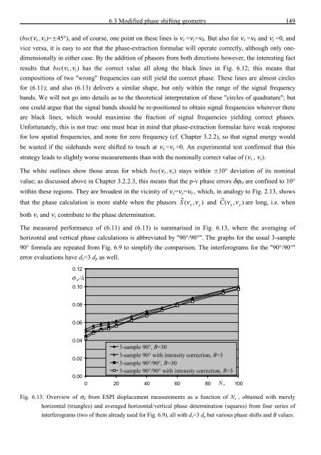
The measured performance <strong>of</strong> (6.11) <strong>and</strong> (6.13) is summarised in Fig. 6.13, where <strong>the</strong> averaging <strong>of</strong><br />
horizontal <strong>and</strong> vertical phase calculations is abbreviated by "90°/90°". The graphs for <strong>the</strong> usual 3-sample<br />
90° formula are repeated from Fig. 6.9 to simplify <strong>the</strong> comparison. The interferograms for <strong>the</strong> "90°/90°"<br />
error evaluations have d s =3 d p as well.<br />
0.12<br />
σ d /λ<br />
0.10<br />
0.08<br />
0.06<br />
0.04<br />
0.02<br />
0.00<br />
3-sample 90°, B=30<br />
3-sample 90° with intensity correction, B=3<br />
3-sample 90°/90°, B=30<br />
3-sample 90°/90° with intensity correction, B=3<br />
0 20 40 60 80 N x 100<br />
Fig. 6.13: Overview <strong>of</strong> σ d from ESPI displacement measurements as a function <strong>of</strong> N x , obtained with merely<br />
horizontal (triangles) <strong>and</strong> averaged horizontal/vertical phase determination (squares) from four series <strong>of</strong><br />
interferograms (two <strong>of</strong> <strong>the</strong>m already used for Fig. 6.9), all with d s =3 d p but various phase shifts <strong>and</strong> B values.


![Skript zur Vorlesung [PDF; 40,0MB ;25.07.2005] - Institut für Physik](https://img.yumpu.com/28425341/1/184x260/skript-zur-vorlesung-pdf-400mb-25072005-institut-fa-1-4-r-physik.jpg?quality=85)


