Application and Optimisation of the Spatial Phase Shifting ...

86 Electronic or Digital Speckle Pattern Interferometry
3.4.4 Spatial phase shifting on speckle fields
We have seen in Fig. 3.21 and Fig. 3.22 that the positive and negative interference bands overlap exactly
in the spatial frequency plane when the source point of the reference wave coincides with the centre of the
aperture. As the origin of the reference wave is laterally displaced, the overlap of the interference spectra
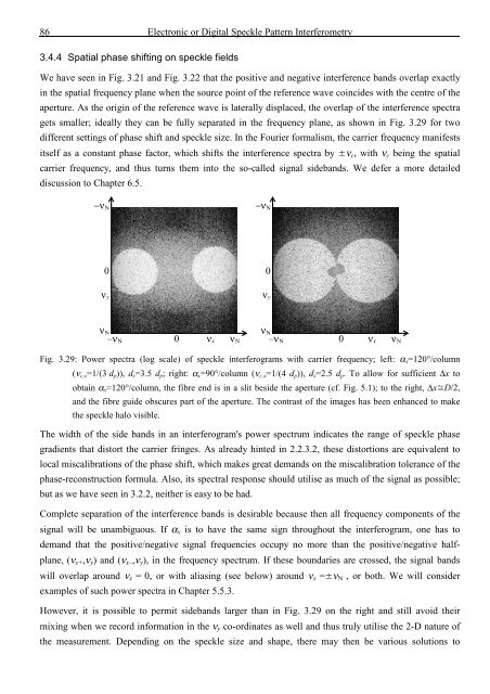
gets smaller; ideally they can be fully separated in the frequency plane, as shown in Fig. 3.29 for two
different settings of phase shift and speckle size. In the Fourier formalism, the carrier frequency manifests
itself as a constant phase factor, which shifts the interference spectra by ν c , with ν c being the spatial
carrier frequency, and thus turns them into the so-called signal sidebands. We defer a more detailed
discussion to Chapter 6.5.
−ν N
0
−ν N
0
ν y
ν y
ν N ν N
–ν N 0 ν x ν N –ν N 0 ν x ν N
Fig. 3.29: Power spectra (log scale) of speckle interferograms with carrier frequency; left: α x =120°/column
(ν c,x =1/(3 d p )), d s =3.5 d p ; right: α x =90°/column (ν c,x =1/(4 d p )), d s =2.5 d p . To allow for sufficient ∆x to
obtain α x =120°/column, the fibre end is in a slit beside the aperture (cf. Fig. 5.1); to the right, ∆x D/2,
and the fibre guide obscures part of the aperture. The contrast of the images has been enhanced to make
the speckle halo visible.
The width of the side bands in an interferogram's power spectrum indicates the range of speckle phase
gradients that distort the carrier fringes. As already hinted in 2.2.3.2, these distortions are equivalent to
local miscalibrations of the phase shift, which makes great demands on the miscalibration tolerance of the
phase-reconstruction formula. Also, its spectral response should utilise as much of the signal as possible;
but as we have seen in 3.2.2, neither is easy to be had.
Complete separation of the interference bands is desirable because then all frequency components of the
signal will be unambiguous. If α x is to have the same sign throughout the interferogram, one has to
demand that the positive/negative signal frequencies occupy no more than the positive/negative halfplane,
(ν x+ ,ν y ) and (ν x– ,ν y ), in the frequency spectrum. If these boundaries are crossed, the signal bands
will overlap around ν x = 0, or with aliasing (see below) around ν x =ν N , or both. We will consider
examples of such power spectra in Chapter 5.5.3.
However, it is possible to permit sidebands larger than in Fig. 3.29 on the right and still avoid their
mixing when we record information in the ν y co-ordinates as well and thus truly utilise the 2-D nature of
the measurement. Depending on the speckle size and shape, there may then be various solutions to