Application and Optimisation of the Spatial Phase Shifting ...

3.3 Temporal phase shifting 77
adding a reference wave [Enn75, Maa98]. To understand how this is meant, we first consider briefly the
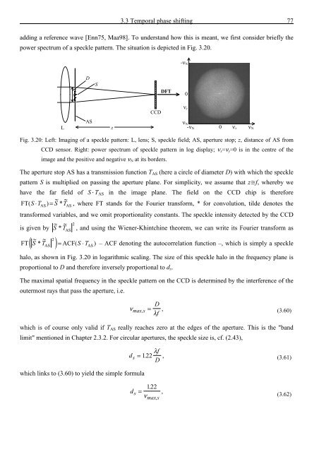
power spectrum of a speckle pattern. The situation is depicted in Fig. 3.20.
−ν N
0
D
S
DFT
L
AS
CCD
z -ν N 0 ν x ν N
ν y
ν N
Fig. 3.20: Left: Imaging of a speckle pattern: L, lens; S, speckle field; AS, aperture stop; z, distance of AS from
CCD sensor. Right: power spectrum of speckle pattern in log display; ν x =ν y =0 is in the centre of the
image and the positive and negative ν N at its borders.
The aperture stop AS has a transmission function T AS (here a circle of diameter D) with which the speckle
pattern S is multiplied on passing the aperture plane. For simplicity, we assume that zf, whereby we
have the far field of ST AS in the image plane. The field on the CCD chip is therefore
~ ~
S ⋅ T ) = S * T , where FT stands for the Fourier transform, * for convolution, tilde denotes the
FT( AS AS
transformed variables, and we omit proportionality constants. The speckle intensity detected by the CCD
is given by S
~ * T ~ 2
AS , and using the Wiener-Khintchine theorem, we can write its Fourier transform as
FT
~ ~
( * AS )
S T 2 = ACF( S ⋅ T ) – ACF denoting the autocorrelation function –, which is simply a speckle
AS
halo, as shown in Fig. 3.20 in logarithmic scaling. The size of this speckle halo in the frequency plane is
proportional to D and therefore inversely proportional to d s .
The maximal spatial frequency in the speckle pattern on the CCD is determined by the interference of the
outermost rays that pass the aperture, i.e.
νmax,s = D λf , (3.60)
which is of course only valid if T AS really reaches zero at the edges of the aperture. This is the "band
limit" mentioned in Chapter 2.3.2. For circular apertures, the speckle size is, cf. (2.43),
d
s = 122 .
which links to (3.60) to yield the simple formula
λ f ,
D
(3.61)
d s
= 122 .
ν
max,s
,
(3.62)