

Application and Optimisation of the Spatial Phase Shifting ...
Application and Optimisation of the Spatial Phase Shifting ...
Application and Optimisation of the Spatial Phase Shifting ...

You also want an ePaper? Increase the reach of your titles
YUMPU automatically turns print PDFs into web optimized ePapers that Google loves.
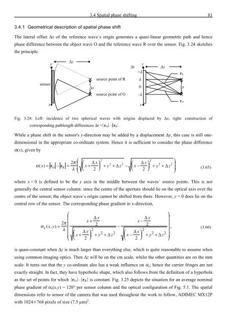
3.4 <strong>Spatial</strong> phase shifting 81<br />
3.4.1 Geometrical description <strong>of</strong> spatial phase shift<br />
The lateral <strong>of</strong>fset ∆x <strong>of</strong> <strong>the</strong> reference wave´s origin generates a quasi-linear geometric path <strong>and</strong> hence<br />
phase difference between <strong>the</strong> object wave O <strong>and</strong> <strong>the</strong> reference wave R over <strong>the</strong> sensor. Fig. 3.24 sketches<br />
<strong>the</strong> principle.<br />
sensor<br />
y<br />
∆z<br />
∆x<br />
source point <strong>of</strong> R<br />
source point <strong>of</strong> O<br />
∆r<br />
y<br />
>λ<br />
λ<br />
0<br />
-λ<br />
∆z<br />
r R<br />
∆x<br />
x<br />
x<br />
r O<br />
Fig. 3.24: Left: incidence <strong>of</strong> two spherical waves with origins displaced by ∆x; right: construction <strong>of</strong><br />
corresponding pathlength differences ∆r = r O – r R .<br />
While a phase shift in <strong>the</strong> sensor's y-direction may be added by a displacement ∆y, this case is still onedimensional<br />
in <strong>the</strong> appropriate co-ordinate system. Hence it is sufficient to consider <strong>the</strong> phase difference<br />
α(x), given by<br />
π ⎛<br />
2<br />
2<br />
2 x<br />
x<br />
α( x)<br />
= − = ⎛ ∆ ⎞<br />
⎜ x + y z x y z<br />
λ ⎝ ⎠<br />
⎟ + − ⎛<br />
⎜<br />
⎝<br />
− ⎞<br />
⎞<br />
2 2<br />
∆<br />
2 2<br />
r r<br />
⎜<br />
⎟ + +<br />
O R<br />
+ ∆<br />
∆<br />
⎝ 2 2 ⎠<br />
⎟<br />
(3.65)<br />
⎠<br />
where x = 0 is defined to be <strong>the</strong> y axis in <strong>the</strong> middle between <strong>the</strong> waves´ source points. This is not<br />
generally <strong>the</strong> central sensor column: since <strong>the</strong> centre <strong>of</strong> <strong>the</strong> aperture should lie on <strong>the</strong> optical axis over <strong>the</strong><br />
centre <strong>of</strong> <strong>the</strong> sensor, <strong>the</strong> object wave´s origin cannot be shifted from <strong>the</strong>re. However, y = 0 does lie on <strong>the</strong><br />
central row <strong>of</strong> <strong>the</strong> sensor. The corresponding phase gradient in x-direction,<br />
⎛<br />
⎜<br />
∆ x<br />
π<br />
x<br />
αx x y 2 ⎜ +<br />
( , ) =<br />
2<br />
⎜<br />
λ<br />
2<br />
⎜ ⎛ ∆ x⎞<br />
⎜ ⎜ x + ⎟ + y<br />
⎝ ⎝ 2 ⎠<br />
2 2<br />
+ ∆ z<br />
−<br />
∆ x<br />
x −<br />
2<br />
2<br />
⎛ ∆ x⎞<br />
⎜ x − ⎟ + y + ∆ z<br />
⎝ 2 ⎠<br />
2 2<br />
⎞<br />
⎟<br />
⎟<br />
⎟ , (3.66)<br />
⎟<br />
⎟<br />
⎠<br />
is quasi-constant when ∆z is much larger than everything else, which is quite reasonable to assume when<br />
using common imaging optics. Then ∆z will be on <strong>the</strong> cm scale, whilst <strong>the</strong> o<strong>the</strong>r quantities are on <strong>the</strong> mm<br />
scale. It turns out that <strong>the</strong> y co-ordinate also has a weak influence on α x ; hence <strong>the</strong> carrier fringes are not<br />
exactly straight. In fact, <strong>the</strong>y have hyperbolic shape, which also follows from <strong>the</strong> definition <strong>of</strong> a hyperbola<br />
as <strong>the</strong> set <strong>of</strong> points for which Fr O F–Fr R F is constant. Fig. 3.25 depicts <strong>the</strong> situation for an average nominal<br />
phase gradient <strong>of</strong> α x (x,y) = 120° per sensor column <strong>and</strong> <strong>the</strong> optical configuration <strong>of</strong> Fig. 5.1. The spatial<br />
dimensions refer to sensor <strong>of</strong> <strong>the</strong> camera that was used throughout <strong>the</strong> work to follow, ADIMEC MX12P<br />
with 1024768 pixels <strong>of</strong> size (7.5 µm) 2 .


![Skript zur Vorlesung [PDF; 40,0MB ;25.07.2005] - Institut für Physik](https://img.yumpu.com/28425341/1/184x260/skript-zur-vorlesung-pdf-400mb-25072005-institut-fa-1-4-r-physik.jpg?quality=85)


