Application and Optimisation of the Spatial Phase Shifting ...

5.6 Impact of light efficiency 131
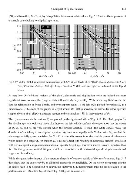
O, and from this, R/O=B, by extrapolation from measurable values. Fig. 5.17 shows the improvement
attainable by switching to elliptical apertures.
0.14
B =1000
14
0.12
12
σ d /λ
0.10
0.08
0.06
B =1000
10
08
06
0.04
0.02
0.00
N x
04
0 0
20 20
50 50
02
100 100
00
0.01 0.1 1 10 100
O I /(µW cm -2 )
N y
0 0
20 20
50 50
100 100
0.01 0.1 1 10 100
O I /(µW cm -2 )
Fig. 5.17: σ d for ESPI displacement measurements with SPS at low levels of O I . "Dark" black: d sx
¡
dsy =3 ¡ 3 d p 2 ;
"bright" white: d sx
¡
dsy =3 ¡ 1 d p 2 . Fringe densities N x (left) and N y (right) as indicated in the legend
boxes.
At very low O I (left-hand regions of the plots), electronic and digitisation noise are indeed the most
significant error sources: the fringe density influences σ d only weakly. With increasing O I however, the
familiar relationship of fringe density and error appears again. To the left, σ d is plotted for various N x as a
function of O I . The slope of the graphs is largest around B=1000 (marked by the arrows for either aperture
shape); the use of an elliptical aperture reduces σ d by as much as 15% in these regions of O I .
The σ d measurements for various N y are plotted on the right-hand side of Fig. 5.17. The black graphs for
the circular aperture look very much like those on the left, which confirms the expectation that the values
of σ d vs. N x and N y are very similar when the circular aperture is used. The white curves reveal the
drawback of switching to an elliptical aperture: σ d rises more rapidly with N y than with N x , so that the
advantage initially gained vanishes for N y >50. Again, this comes from the speckle pattern displacement
which results in a larger σ d for smaller d s . Thus for object tilts resulting in horizontal fringes (associated
with vertical speckle displacements and small speckle height d sy ), this error source is more important than
for tilts that generate vertical fringes, which are associated with horizontal speckle displacements and
large speckle width d sx .
While the quantitative impact of the aperture shape is of course specific of the interferometer, Fig. 5.17
does show that the anisotropy by an elliptical aperture is not negligible. On the whole, the greater amount
of light is seen to be helpful; but of course, the improved SPS measurement must be set in relation to the
performance of TPS at low O I , of which Fig. 5.18 gives an overview.