Application and Optimisation of the Spatial Phase Shifting ...

2.3 Second-order speckle statistics 37
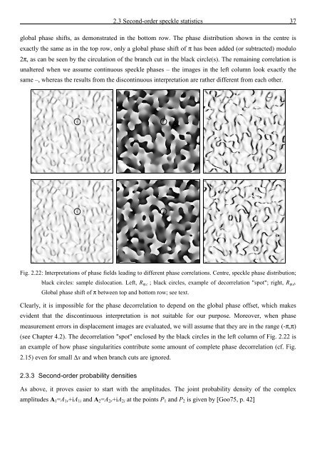
global phase shifts, as demonstrated in the bottom row. The phase distribution shown in the centre is
exactly the same as in the top row, only a global phase shift of π has been added (or subtracted) modulo
2π, as can be seen by the circulation of the branch cut in the black circle(s). The remaining correlation is
unaltered when we assume continuous speckle phases – the images in the left column look exactly the
same –, whereas the results from the discontinuous interpretation are rather different from each other.
Fig. 2.22: Interpretations of phase fields leading to different phase correlations. Centre, speckle phase distribution;
black circles: sample dislocation. Left, R ϕ,c ; black circles, example of decorrelation "spot"; right, R ϕ,d .
Global phase shift of π between top and bottom row; see text.
Clearly, it is impossible for the phase decorrelation to depend on the global phase offset, which makes
evident that the discontinuous interpretation is not suitable for our purpose. Moreover, when phase
measurement errors in displacement images are evaluated, we will assume that they are in the range (-π,π)
(see Chapter 4.2). The decorrelation "spot" enclosed by the black circles in the left column of Fig. 2.22 is
an example of how phase singularities contribute some amount of complete phase decorrelation (cf. Fig.
2.15) even for small ∆x and when branch cuts are ignored.
2.3.3 Second-order probability densities
As above, it proves easier to start with the amplitudes. The joint probability density of the complex
amplitudes A 1 =A 1r +iA 1i and A 2 =A 2r +iA 2i at the points P 1 and P 2 is given by [Goo75, p. 42]