Application and Optimisation of the Spatial Phase Shifting ...

More documents

Recommendations

Info

156 Improvements on SPS generally necessary in speckle interferometry (nevertheless, it may sometimes be useful to inspect the speckle phases per se). In classical interferometry, the variations of the background intensity may reasonably be assumed to be so low-frequent that the spectrum of the variations of I b is easily separated from the signal in frequency space. In speckle interferometry however, the high frequencies in O(x,y) cause a significant deficiency of the FTM: as is clearly seen from Fig. 6.17, O ~ ( ν x , ν y ) is not separated from the sidebands. The speckle halo overlaps the sidebands at any practicable speckle size, so that a considerable noise background adds to most of the signal's frequency content. This disturbs the phase reconstruction in a similar way as in the phase-shifting investigations. But as familiar as the problems are the ways to cope with them. From (6.19), it is clear that increasing B will again help to suppress the speckle noise, provided r(x,y) has a narrow spectrum and can be eliminated in the frequency plane. This can be fulfilled in an excellent way if a fibre is used to illuminate the sensor: then r(x,y) will be a very broad Gaussian profile, and its spectrum a very narrow Gaussian that will not overlap with the signal sidebands. It turns out that the performance of the FTM depends on B much in the same way as for the phase-sampling methods. To quantify this, Fig. 6.1 also contains a plot of σ d as calculated by (6.19) -(6.21) (black, circle symbols) from the same interferograms as used for the SPS tests. Furthermore, we note that the quantity O ~ ( ν x , ν y ) in (6.19) is directly accessible because of ~ O ( νx , ν y ) = FT O ( x , y ) = FT o ( x , y ) o ( x , y ) , (6.22) * ( ) ( ) so that we should be able to eliminate the speckle background from the phase calculation if we first record the speckle pattern alone, calculate its spectrum and subtract it from (6.18). This correction for speckle intensity is similar to that in 6.2.1, and the remaining phase errors are then mainly from electronic noise and pixels with insufficient M I . The same would be possible for the reference wave if its spectrum would overlap the signal spectra. This approach resembles the background subtraction suggested in [Liu97] for classical interferometry. Using the linearity of the Fourier transform, we could even subtract the speckle pattern in the space domain (6.17) before switching to the frequency domain; but the benefit is easier to see in the frequency representation. Fig. 6.18 provides an example of how the speckle noise is removed in the Fourier plane when d s =2 d p . The aliased frequencies over ν N remain usable for the FTM by pasting them back to where they got cut off [Bon86]. The reference wave need not be accounted for, since its spectrum is indeed easily separated from the sidebands.
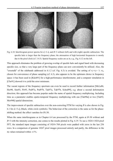
6.5 Fourier transform method of phase determination 157 Fig. 6.18: Interferogram power spectra for d s =2 d p and B=3 without (left) and with (right) speckle subtraction. The speckle halo is larger than the frequency plane; the attenuation of high horizontal frequencies is mostly due to the pixel clock (cf. 3.4.5). Spatial frequency scales are as in, e.g., Fig. 6.12 on the left. This approach eliminates the problem of growing overlap of speckle halo and signal band with decreasing speckle size, so that a very large part of the frequency plane can now conveniently be utilised. Also, the "crosstalk" of the sidebands addressed in 6.1.2 (cf. Fig. 6.3) is avoided. The setting of ν x =ν y = ½ ν N , chosen for convenience of phase sampling (cf. 6.3), also appears to be the optimum choice in frequency space: it has been used in [Küch91] for a high-performance interferometer, and a computer simulation in [Che91] showed it to yield the error minimum. The vacant regions of the frequency spectrum can even be used to record further information [McLa86, Hor90, Sim93, Pir95, Ped97a, Ped97b, Tak97a, Tak97b, Sched99], e.g. about a second deformation direction; this approach has become popular under the name of spatial frequency multiplexing. Including time as a parameter enables spatio-temporal frequency multiplexing with one [Tak90a] or two [Tak92, Mor94b] spatial dimensions. The improvement of speckle subtraction over the non-correcting FTM for varying B is also shown in Fig. 6.1 for d s =3 d p (black, white circle symbols). The behaviour of the correction is the same as for the phaseshifting method: the effect vanishes for B30. When the same interferograms as in Chapter 6.4 are processed by the FTM, again at B=30 without and B=3 with the intensity correction, one comes to the results plotted in Fig. 6.19. To use a 10241024 pixel FFT, the standard input images consisting of 1024768 pixels were padded with zeros in the last 256 rows. In a comparison of genuine 1024 2 pixel images processed entirely and partly, the difference in the σ d values remained within 1%.
Page 1 and 2:
Application and Optimisation of the
Page 3 and 4:
Table of Contents 1 1 INTRODUCTION
Page 5 and 6:
3 1 Introduction The present era of
Page 7 and 8:
Introduction 5 retrieval can help t
Page 9 and 10:
7 2 Statistical Properties of Speck
Page 11 and 12:
2.1 Experimental set-up 9 Gaussian
Page 13 and 14:
2.2 First-order speckle statistics
Page 15 and 16:
Page 17 and 18:
Page 19 and 20:
Page 21 and 22:
Page 23 and 24:
Page 25 and 26:
Page 27 and 28:
Page 29 and 30:
Page 31 and 32:
Page 33 and 34:
Page 35 and 36:
2.3 Second-order speckle statistics
Page 37 and 38:
Page 39 and 40:
Page 41 and 42:
Page 43 and 44:
Page 45 and 46:
Page 47 and 48:
Page 49 and 50:
47 3 Electronic or Digital Speckle
Page 51 and 52:
3.1 Subtraction-mode ESPI 49 some 4
Page 53 and 54:
3.2 Phase-shifting ESPI 51 filled u
Page 55 and 56:
3.2 Phase-shifting ESPI 53 known si
Page 57 and 58:
3.2 Phase-shifting ESPI 55 α n =α
Page 59 and 60:
3.2 Phase-shifting ESPI 57 But reme
Page 61 and 62:
3.2 Phase-shifting ESPI 59 ϕ ϕ O,
Page 63 and 64:
3.2 Phase-shifting ESPI 61 These fo
Page 65 and 66:
3.2 Phase-shifting ESPI 63 ∞ ~ ~
Page 67 and 68:
3.2 Phase-shifting ESPI 65 ∞ N
Page 69 and 70:
3.2 Phase-shifting ESPI 67 The spec
Page 71 and 72:
3.2 Phase-shifting ESPI 69 − 0. 2
Page 73 and 74:
3.2 Phase-shifting ESPI 71 ν x 0 i
Page 75 and 76:
3.2 Phase-shifting ESPI 73 to think
Page 77 and 78:
3.3 Temporal phase shifting 75 Agai
Page 79 and 80:
3.3 Temporal phase shifting 77 addi
Page 81 and 82:
3.4 Spatial phase shifting 79 which
Page 83 and 84:
3.4 Spatial phase shifting 81 3.4.1
Page 85 and 86:
3.4 Spatial phase shifting 83 cross
Page 87 and 88:
3.4 Spatial phase shifting 85 Fig.
Page 89 and 90:
3.4 Spatial phase shifting 87 arran
Page 91 and 92:
3.4 Spatial phase shifting 89 infor
Page 93 and 94:
3.4 Spatial phase shifting 91 frequ
Page 95 and 96:
3.4 Spatial phase shifting 93 altho
Page 97 and 98:
3.4 Spatial phase shifting 95 error
Page 99:
3.4 Spatial phase shifting 97 Since
Page 102 and 103:
100 Quantification of displacement-
Page 104 and 105:
Page 106 and 107:
Page 108 and 109: 106 Quantification of displacement-
Page 110 and 111: 108 Quantification of displacement-
Page 112 and 113: 110
Page 114 and 115: 112 Comparison of noise in phase ma
Page 136 and 137: 134 Improvements on SPS intensity o
Page 138 and 139: 136 Improvements on SPS 0.14 σ d /
Page 140 and 141: 138 Improvements on SPS we are conc
Page 142 and 143: 140 Improvements on SPS 6.2 Modifie
Page 146 and 147: 144 Improvements on SPS Fig. 6.7 te
Page 148 and 149: 146 Improvements on SPS Finally, bo
Page 150 and 151: 148 Improvements on SPS To use the
Page 152 and 153: 150 Improvements on SPS The improve
Page 154 and 155: 152 Improvements on SPS On the whol
Page 156 and 157: 154 Improvements on SPS In classica
Page 162 and 163: 160 Improvements on SPS uncertain,
Page 164 and 165: 162 Improvements on SPS To obtain p
Page 166 and 167: 164 Improvements on SPS Fig. 6.22:
Page 168 and 169: 166 Improvements on SPS This proced
Page 170 and 171: 168 Improvements on SPS 6.7.2 Long-
Page 172 and 173: 170 Improvements on SPS Fig. 6.28:
Page 174 and 175: 172 Improvements on SPS the heater
Page 176 and 177: 174
Page 178 and 179: 176 Summary method to search for a
Page 180 and 181: 178
Page 182 and 183: 180 References [Bot97] [Bra87] [Bro
Page 184 and 185: 182 References [Ett97] [Fac93] [Far
Page 186 and 187: 184 References [Har94] [Her96] [Het
Page 188 and 189: 186 References [Kuj89] [Kuj91a] [Ku
Page 190 and 191: 188 References [McLa86] [Mer83] J.
Page 192 and 193: 190 References [Rav99] I. Raveh, E.
Page 194 and 195: 192 References [Sur98b] [Sur98c] [S
Page 196 and 197: 194
Page 198 and 199: 196 Appendix A: Counting events and
Page 200 and 201: 198 Appendix B: Real-time phase cal
Page 202 and 203: 200 Appendix C: Derivation of inten
Page 204 and 205: I 1 a r g ( S ~ ( ) ) 202 Appendix
Page 206 and 207: 204 Appendix D: Alternative error-c
Page 208 and 209:
206
Page 210 and 211:
208
Page 212 and 213:
210 The author List of publications
Page 214:
212
show all

Application and Optimisation of the Spatial Phase Shifting ...

Create successful ePaper yourself

Delete template?

Save as template?