Application and Optimisation of the Spatial Phase Shifting ...

74 Electronic or Digital Speckle Pattern Interferometry
It is also possible to average two 4-step formulae [Schwi83, Har87], which yields a 4+1 formula, or to
extend the averaging approach to even more samples [Schmi95a, Zha99]. Particularly the 4+1 formula is
very frequently used in ESPI; but we ignore it here because it requires 5 samples already; we will briefly
discuss 5-sample formulae in Appendix D.
While formulae with α=90° are most effective against detuning due to the error frequency having twice
the signal frequency, it is also possible to design compensating formulae with α=120°. A recipe to do so
has been given in [Lar92b]; it is based on arranging the a n and b n (anti)symmetrically over the sampling
sequence (which results in frequency-independent quadrature) and matching the gradients of S ~ ( ν ) and
~ C( ν)
at ν0 . (At this point, we note that also (3.56) fulfils these criteria; in fact, all the formulae with stable
quadrature presented thus far have (anti)symmetrically arranged coefficients. This so-called Hermitian
symmetry of the coefficients is a necessary and sufficient condition for the frequency independence of the
quadrature, and it has been shown in [Sur98a, Hib98] how to symmetrise phase-shifting formulae.)
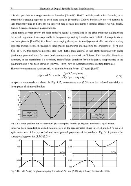
The error-compensating symmetrical 3+1-sample formula for α=120° reads [Lar99]
ϕ
O
mod 2π
= arctan
I0 + 3( I1 − I2)
− I3
3( − I + I + I − I ) ; (3.58)
0 1 2 3
its spectral characteristics, shown in Fig. 3.17, demonstrate that (3.58) also has reduced sensitivity to
linear phase-shift miscalibration.
6
3.14
4
2
1.57
0
0 1 2 3
-2
-4
-6
amp( S
~ ( νx))
amp( C
~ ( ν x ))
ν x /ν 0x
0
-1.57
-3.14
0 1 2 3
arg( S
~ ( νx))
arg( C
~ ( ν x ))
Fig. 3.17: Filter spectrum for 3+1-step-120° phase-sampling formula (3.58); left: amplitudes, right: phases.
Since we have been dealing with different offsets of the reconstructed phase in (3.56) and (3.57), we will
again make use of bsc(ν x ) to find out more general properties of the methods. Fig. 3.18 presents the
corresponding plots for (3.56)-(3.58).
1.57
1.57
ν x /ν 0x
0.785
0.785
ν x /ν 0x
-1.57
0
-0.785
0 1 2 3 0 4
-0.785
ν x /ν 0x
0
0 1 2 3
-1.57
Fig. 3.18: Left: bsc(ν) for phase-sampling formulae (3.56) and (3.57); right: bsc(ν) for formula (3.58).