Application and Optimisation of the Spatial Phase Shifting ...

3.4 Spatial phase shifting 89
information about the actual manipulation of the interferogram's frequency content by the phase
calculation.
The phase lag between the "sine" and "cosine" fringe patterns may be estimated when we determine their
phases as if they were interferograms and then subtract these phase maps as if we wanted to measure a
deformation. The "double" phase determination of course leads to a circular argument, which we must
avoid by using the Fourier-transform method (cf. Chapter 6.5).
To valuate the spectral transfer characteristics of phase-shifting formulae, we could simply choose white
noise, e.g. a random distribution of grey values, as a dummy interferogram for input; but since our
objective here is an experimental check of the findings in 3.2.2, we use actual interferograms. Starting
with α=90°, we choose the interferogram with the spectrum of Fig. 3.29 (right side) as input, which
indeed accounts for the whole range of interest, ν x =0 up to ν x =ν N . The power spectra that we compare are
scaled linearly this time to fit the expected deviations; the low-frequency part of the spectra then has to be
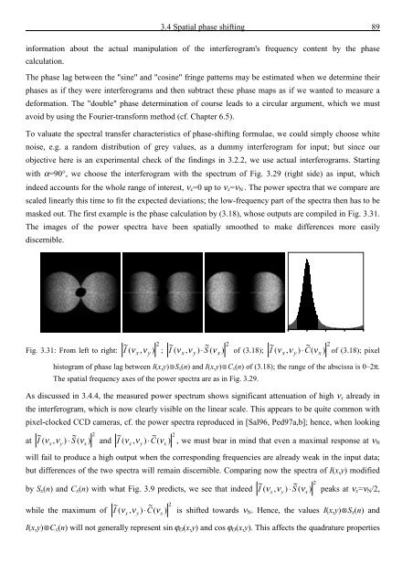
masked out. The first example is the phase calculation by (3.18), whose outputs are compiled in Fig. 3.31.
The images of the power spectra have been spatially smoothed to make differences more easily
discernible.
Fig. 3.31: From left to right: ~ 2 ~ ~ 2 ~ ~ 2
( ν , ν ) ; I ( ν , ν ) ⋅ S ( ν ) of (3.18); I ( ν , ν ) ⋅ C(
ν ) of (3.18); pixel
I x y
x y x
x y x
histogram of phase lag between I(x,y) S x (n) and I(x,y) C x (n) of (3.18); the range of the abscissa is 0–2π.
The spatial frequency axes of the power spectra are as in Fig. 3.29.
As discussed in 3.4.4, the measured power spectrum shows significant attenuation of high ν x already in
the interferogram, which is now clearly visible on the linear scale. This appears to be quite common with
pixel-clocked CCD cameras, cf. the power spectra reproduced in [Sal96, Ped97a,b]; hence, when looking
at ~ ~
2
~ ~ 2
I ( ν , ν ) ⋅ S ( ν ) and I ( ν , ν ) ⋅ C(
ν ) , we must bear in mind that even a maximal response at νN
x y x
x y x
will fail to produce a high output when the corresponding frequencies are already weak in the input data;
but differences of the two spectra will remain discernible. Comparing now the spectra of I(x,y) modified
by S x (n) and C x (n) with what Fig. 3.9 predicts, we see that indeed ~ ~ 2
I ( ν , ν ) ⋅ S ( ν ) peaks at νx =ν N /2,
x y x
while the maximum of ~ ( , ) ~ 2
I ν ν ⋅C( ν ) is shifted towards νN . Hence, the values I(x,y)S x (n) and
x y x
I(x,y)C x (n) will not generally represent sin ϕ O (x,y) and cos ϕ O (x,y). This affects the quadrature properties