Application and Optimisation of the Spatial Phase Shifting ...

I
1
a r g (
S
~
( ) )
202 Appendix D: Alternative error-compensating formulae
The sampling window thus defined offers excellent phase-shift error suppression while sacrificing only
little spatial resolution; it has been pointed out in [Küch91] that the slant of the carrier fringes saves a
factor of L2 in this respect.
It is also possible to make all three points of zero error coincide at α=90°/sample, which was already
remarked in [Küch91] and later derived independently by [MYo95, Schmi95a]; in this case the phase
calculation is very stable around α=90° but does not reach zero error again when α≠90°. The
corresponding sampling formula reads
ϕ
O
− I0 + 4( I1 − I3)
+ I4
mod 2π
= arctan
− I − 2I + 6I − 2I − I
and the corresponding filter spectrum is shown in Fig. D.3.
0 1 2 3 4
,
(D.2)
9
3.14
6
3
1.57
0
-3
-6
-9
0 1 2 3
n/n 0 4
amp( S
~ ( ν ))
xy
amp( C
~ ( ν ))
xy
ν ξψ
/ν 0
0
-1.57
-3.14
ν ξψ
/ν 0
0 1 2 3 4
ν xy
arg( C
~ ( ν ))
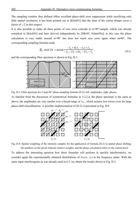
Fig. D.3: Filter spectrum for 5-step-90° phase-sampling formula (D.2); left: amplitudes, right: phases.
As familiar from the discussion of symmetrical formulae in 3.2.2.4, the phase spectrum is the same as
above; the amplitudes are very similar over a broad range of ν xy , which assures low errors even for large
phase-shift miscalibration. A possible implementation of (D.2) is presented in Fig. D.4.
xy
ϕ O
–180°
ϕ O
–90°
ϕ O
–1
2
2 0
0
2
ϕ O
+90°
ϕ O
+180°
–1
–1
–1 1
4
–1
0
2
–1
1
–1
–1
S xy( n) C xy( n)
Fig. D.4: Spatial weighting of the intensity samples for the application of formula (D.2) in spatial phase shifting;
the numbers on the pixels indicate relative weights, and the phase calculation refers to the central pixel.
To address the interesting question how these formulae will perform in speckle interferometry, we
consider again the experimentally obtained distributions of bsc(ν x ,ν y ) in the frequency plane. With the
same input interferogram as was already used in 6.3, we obtain the results shown in Fig. D.5.