Application and Optimisation of the Spatial Phase Shifting ...

122 Comparison of noise in phase maps from TPS and SPS
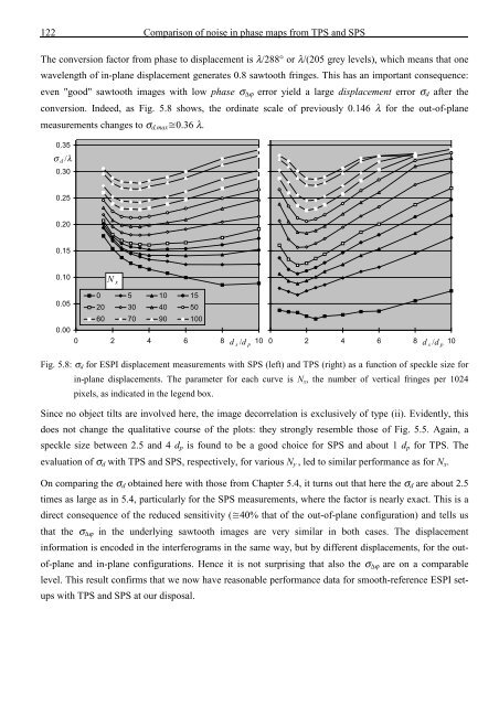
The conversion factor from phase to displacement is λ/288° or λ/(205 grey levels), which means that one
wavelength of in-plane displacement generates 0.8 sawtooth fringes. This has an important consequence:
even "good" sawtooth images with low phase σ ∆ϕ error yield a large displacement error σ d after the
conversion. Indeed, as Fig. 5.8 shows, the ordinate scale of previously 0.146 λ for the out-of-plane
measurements changes to σ d,max 0.36 λ.
0.35
σ d /λ
0.30
5
0
0.25
5
0.20
0
0.15
5
0.10
0
0.05
0.00
N x
0 5 10 15
20 30 40 50
5
60 70 90 100
0
0 2 4 6 8 d s /d p
10
0 2 4 6 8 d s /d p
10
Fig. 5.8: σ d for ESPI displacement measurements with SPS (left) and TPS (right) as a function of speckle size for
in-plane displacements. The parameter for each curve is N x , the number of vertical fringes per 1024
pixels, as indicated in the legend box.
Since no object tilts are involved here, the image decorrelation is exclusively of type (ii). Evidently, this
does not change the qualitative course of the plots: they strongly resemble those of Fig. 5.5. Again, a
speckle size between 2.5 and 4 d p is found to be a good choice for SPS and about 1 d p for TPS. The
evaluation of σ d with TPS and SPS, respectively, for various N y , led to similar performance as for N x .
On comparing the σ d obtained here with those from Chapter 5.4, it turns out that here the σ d are about 2.5
times as large as in 5.4, particularly for the SPS measurements, where the factor is nearly exact. This is a
direct consequence of the reduced sensitivity (40% that of the out-of-plane configuration) and tells us
that the σ ∆ϕ in the underlying sawtooth images are very similar in both cases. The displacement
information is encoded in the interferograms in the same way, but by different displacements, for the outof-plane
and in-plane configurations. Hence it is not surprising that also the σ ∆ϕ are on a comparable
level. This result confirms that we now have reasonable performance data for smooth-reference ESPI setups
with TPS and SPS at our disposal.