- Page 2:
The Logic of Scientific Discovery
- Page 5 and 6:
Logik der Forschung first published
- Page 8 and 9:
CONTENTS Translators’ Note xii Pr
- Page 10 and 11:
contents ix 7 37 Logical Ranges. No
- Page 12 and 13:
iii Derivation of the First Form of
- Page 14 and 15:
translators’ note xiii In these n
- Page 16 and 17:
PREFACE TO THE FIRST EDITION, 1934
- Page 18 and 19:
There is nothing more necessary to
- Page 20 and 21:
preface, 1959 xix Language analysts
- Page 22 and 23:
xxii preface, 1959 perception or kn
- Page 24 and 25:
preface, 1959 xxiii essence of phil
- Page 26 and 27:
preface, 1959 xxv elaborate and fam
- Page 28:
ACKNOWLEDGMENTS, 1960 and 1968 I wi
- Page 32 and 33:
1 A SURVEY OF SOME FUNDAMENTAL PROB
- Page 34 and 35:
a survey of some fundamental proble
- Page 36 and 37:
a survey of some fundamental proble
- Page 38 and 39:
a survey of some fundamental proble
- Page 40 and 41:
a survey of some fundamental proble
- Page 42 and 43:
trivial; for metaphysics has usuall
- Page 44 and 45:
a survey of some fundamental proble
- Page 46 and 47:
non-contradictory, a possible world
- Page 48 and 49:
a survey of some fundamental proble
- Page 50 and 51:
a survey of some fundamental proble
- Page 52 and 53:
a survey of some fundamental proble
- Page 54 and 55:
a survey of some fundamental proble
- Page 56 and 57:
2 ON THE PROBLEM OF A THEORY OF SCI
- Page 58 and 59:
on the problem of a theory of scien
- Page 60 and 61:
on the problem of a theory of scien
- Page 62 and 63:
on the problem of a theory of scien
- Page 64:
Part II Some Structural Components
- Page 67 and 68:
38 some structural components of a
- Page 69 and 70:
40 some structural components of a
- Page 71 and 72:
42 some structural components of a
- Page 73 and 74:
44 some structural components of a
- Page 75 and 76:
46 some structural components of a
- Page 77 and 78:
48 some structural components of a
- Page 79 and 80:
50 some structural components of a
- Page 81 and 82:
52 some structural components of a
- Page 83 and 84:
54 some structural components of a
- Page 85 and 86:
56 some structural components of a
- Page 87 and 88:
58 some structural components of a
- Page 89 and 90:
60 some structural components of a
- Page 91 and 92:
62 some structural components of a
- Page 93 and 94:
64 some structural components of a
- Page 95 and 96:
66 some structural components of a
- Page 97 and 98:
68 some structural components of a
- Page 99 and 100:
70 some structural components of a
- Page 101 and 102:
72 some structural components of a
- Page 103 and 104:
5 THE PROBLEM OF THE EMPIRICAL BASI
- Page 105 and 106:
76 some structural components of a
- Page 107 and 108:
78 some structural components of a
- Page 109 and 110:
80 some structural components of a
- Page 111 and 112:
82 some structural components of a
- Page 113 and 114:
84 some structural components of a
- Page 115 and 116:
86 some structural components of a
- Page 117 and 118:
88 some structural components of a
- Page 119 and 120:
90 some structural components of a
- Page 121 and 122:
92 some structural components of a
- Page 123 and 124:
94 some structural components of a
- Page 125 and 126:
96 some structural components of a
- Page 127 and 128:
98 some structural components of a
- Page 129 and 130:
100 some structural components of a
- Page 131 and 132:
102 some structural components of a
- Page 133 and 134:
104 some structural components of a
- Page 135 and 136:
106 some structural components of a
- Page 137 and 138:
108 some structural components of a
- Page 139 and 140:
110 some structural components of a
- Page 141 and 142:
112 some structural components of a
- Page 143 and 144:
114 some structural components of a
- Page 145 and 146:
116 some structural components of a
- Page 147 and 148:
118 some structural components of a
- Page 149 and 150:
120 some structural components of a
- Page 151 and 152:
122 some structural components of a
- Page 153 and 154:
124 some structural components of a
- Page 155 and 156:
126 some structural components of a
- Page 157 and 158:
128 some structural components of a
- Page 159 and 160:
130 some structural components of a
- Page 161 and 162:
132 some structural components of a
- Page 163 and 164:
134 some structural components of a
- Page 165 and 166:
136 some structural components of a
- Page 167 and 168:
138 some structural components of a
- Page 169 and 170:
140 some structural components of a
- Page 171 and 172:
142 some structural components of a
- Page 173 and 174:
144 some structural components of a
- Page 175 and 176:
146 some structural components of a
- Page 177 and 178:
148 some structural components of a
- Page 179 and 180:
150 some structural components of a
- Page 181 and 182:
152 some structural components of a
- Page 183 and 184:
154 some structural components of a
- Page 185 and 186:
156 some structural components of a
- Page 187 and 188:
158 some structural components of a
- Page 189 and 190:
160 some structural components of a
- Page 191 and 192:
162 some structural components of a
- Page 193 and 194:
164 some structural components of a
- Page 195 and 196:
166 some structural components of a
- Page 197 and 198:
168 some structural components of a
- Page 199 and 200:
170 some structural components of a
- Page 201 and 202:
172 some structural components of a
- Page 203 and 204:
174 some structural components of a
- Page 205 and 206:
176 some structural components of a
- Page 207 and 208:
178 some structural components of a
- Page 209 and 210:
180 some structural components of a
- Page 211 and 212:
182 some structural components of a
- Page 213 and 214:
184 some structural components of a
- Page 215 and 216:
186 some structural components of a
- Page 217 and 218:
188 some structural components of a
- Page 219 and 220:
190 some structural components of a
- Page 221 and 222:
192 some structural components of a
- Page 223 and 224:
194 some structural components of a
- Page 225 and 226:
196 some structural components of a
- Page 227 and 228:
198 some structural components of a
- Page 229 and 230:
200 some structural components of a
- Page 231 and 232:
202 some structural components of a
- Page 233 and 234:
204 some structural components of a
- Page 235 and 236:
206 some structural components of a
- Page 237 and 238:
208 some structural components of a
- Page 239 and 240:
210 some structural components of a
- Page 241 and 242:
212 some structural components of a
- Page 243 and 244:
214 some structural components of a
- Page 245 and 246:
216 some structural components of a
- Page 247 and 248:
218 some structural components of a
- Page 249 and 250:
220 some structural components of a
- Page 251 and 252:
222 some structural components of a
- Page 253 and 254:
224 some structural components of a
- Page 255 and 256:
226 some structural components of a
- Page 257 and 258:
228 some structural components of a
- Page 259 and 260:
230 some structural components of a
- Page 261 and 262:
232 some structural components of a
- Page 263 and 264:
234 some structural components of a
- Page 265 and 266:
236 some structural components of a
- Page 267 and 268:
238 some structural components of a
- Page 269 and 270:
240 some structural components of a
- Page 271 and 272:
242 some structural components of a
- Page 273 and 274:
244 some structural components of a
- Page 275 and 276:
246 some structural components of a
- Page 277 and 278:
10 CORROBORATION, OR HOW A THEORY S
- Page 279 and 280:
250 some structural components of a
- Page 281 and 282:
252 some structural components of a
- Page 283 and 284:
254 some structural components of a
- Page 285 and 286:
256 some structural components of a
- Page 287 and 288:
258 some structural components of a
- Page 289 and 290:
260 some structural components of a
- Page 291 and 292:
262 some structural components of a
- Page 293 and 294:
264 some structural components of a
- Page 295 and 296:
266 some structural components of a
- Page 297 and 298:
268 some structural components of a
- Page 299 and 300:
270 some structural components of a
- Page 301 and 302:
272 some structural components of a
- Page 303 and 304:
274 some structural components of a
- Page 305 and 306:
276 some structural components of a
- Page 307 and 308:
278 some structural components of a
- Page 309 and 310:
280 some structural components of a
- Page 311 and 312:
282 some structural components of a
- Page 313 and 314:
284 appendices it is connected with
- Page 315 and 316:
APPENDIX ii The General Calculus of
- Page 317 and 318:
288 appendices —we obtain from (2
- Page 319 and 320:
APPENDIX iii Derivation of the Firs
- Page 321 and 322:
292 appendices (6,1) αF″(σ´ m.
- Page 323 and 324:
294 appendices after effect) in the
- Page 325 and 326:
296 appendices (b) An analogous met
- Page 327 and 328:
298 appendices position), then we a
- Page 329 and 330:
300 appendices incoherent photons.
- Page 331 and 332:
302 appendices interposition of a f
- Page 333 and 334:
304 appendices wave-packets (obtain
- Page 335 and 336:
306 appendices slit. This angle φ
- Page 337 and 338:
308 appendices latter, if we use hi
- Page 339 and 340:
310 new appendices The first two of
- Page 341 and 342:
APPENDIX *i Two Notes on Induction
- Page 343 and 344:
314 new appendices statements’;*
- Page 345 and 346:
316 new appendices be the source fr
- Page 347 and 348:
318 new appendices with the help of
- Page 349 and 350:
320 new appendices logical interpre
- Page 351 and 352:
322 new appendices It is desirable
- Page 353 and 354:
324 new appendices operations—con
- Page 355 and 356:
326 new appendices (3) It will be a
- Page 357 and 358:
328 new appendices (7) The derivati
- Page 359 and 360:
330 new appendices There are three
- Page 361 and 362:
332 new appendices that is to say,
- Page 363 and 364:
334 new appendices invalid, and sho
- Page 365 and 366:
336 new appendices simplified syste
- Page 367 and 368:
338 new appendices The following co
- Page 369 and 370:
340 new appendices able to show tha
- Page 371 and 372:
342 new appendices obtain p(a, c) =
- Page 373 and 374:
344 new appendices The second examp
- Page 375 and 376:
346 new appendices first consistenc
- Page 377 and 378:
348 new appendices S′ ={0, 1, 2,
- Page 379 and 380:
350 new appendices B1 is violated b
- Page 381 and 382:
352 new appendices always fill the
- Page 383 and 384:
354 new appendices It should be men
- Page 385 and 386:
APPENDIX *v Derivations in the Form
- Page 387 and 388:
358 new appendices (26) (Eb) (Ea) p
- Page 389 and 390:
360 new appendices (Applying B2 twi
- Page 391 and 392:
362 new appendices form: it is unco
- Page 393 and 394:
364 new appendices In order to prov
- Page 395 and 396:
366 new appendices which is neverth
- Page 397 and 398:
368 new appendices the other axioms
- Page 399 and 400:
370 new appendices between rain and
- Page 401 and 402:
372 new appendices in the widest po
- Page 403 and 404:
APPENDIX *vii Zero Probability and
- Page 405 and 406:
376 new appendices favourable possi
- Page 407 and 408:
378 new appendices (4) p(a) = lim p
- Page 409 and 410: 380 new appendices The same point m
- Page 411 and 412: 382 new appendices inferences from
- Page 413 and 414: 384 new appendices the required a a
- Page 415 and 416: 386 new appendices ‘universe’
- Page 417 and 418: 388 new appendices All this does no
- Page 419 and 420: 390 new appendices The fine-structu
- Page 421 and 422: APPENDIX *viii Content, Simplicity,
- Page 423 and 424: 394 new appendices each entry repre
- Page 425 and 426: 396 new appendices But formula (*)
- Page 427 and 428: 398 new appendices (−) d(a 1)p(a
- Page 429 and 430: 400 new appendices thus becomes som
- Page 431 and 432: APPENDIX *ix Corroboration, the Wei
- Page 433 and 434: 404 new appendices I will now brief
- Page 435 and 436: 406 new appendices of the brevity o
- Page 437 and 438: 408 new appendices who identify, ex
- Page 439 and 440: 410 new appendices Kemeny.) Therefo
- Page 441 and 442: 412 new appendices DEGREE OF CONFIR
- Page 443 and 444: 414 new appendices (4.5) C(x 1x 2 o
- Page 445 and 446: 416 new appendices strongly upon P(
- Page 447 and 448: 418 new appendices (vii) If C(x) =
- Page 449 and 450: 420 new appendices to be slightly a
- Page 451 and 452: 422 new appendices length, to take
- Page 453 and 454: 424 new appendices A THIRD NOTE ON
- Page 455 and 456: 426 new appendices (3) P(a) = P(a,
- Page 457 and 458: 428 new appendices behaviour of E a
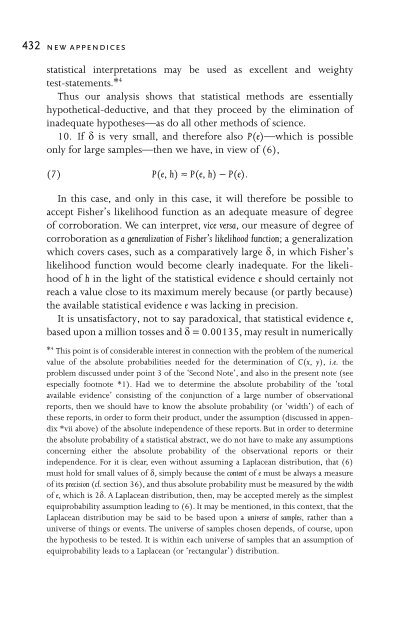
- Page 459: 430 new appendices either if δ is
- Page 463 and 464: 434 new appendices them, there is a
- Page 465 and 466: 436 new appendices statements e, f,
- Page 467 and 468: 438 new appendices simply deceive o
- Page 469 and 470: APPENDIX *x Universals, Disposition
- Page 471 and 472: 442 new appendices One can easily s
- Page 473 and 474: 444 new appendices statement such a
- Page 475 and 476: 446 new appendices more abstract. T
- Page 477 and 478: 448 new appendices natural laws see
- Page 479 and 480: 450 new appendices indirect proof.
- Page 481 and 482: 452 new appendices physical theory
- Page 483 and 484: 454 new appendices is deducible fro
- Page 485 and 486: 456 new appendices A little reflect
- Page 487 and 488: 458 new appendices differ (if at al
- Page 489 and 490: 460 new appendices the world. And a
- Page 491 and 492: 462 new appendices the phenomenalis
- Page 493 and 494: APPENDIX *xi On the Use and Misuse
- Page 495 and 496: 466 new appendices a gravitational
- Page 497 and 498: 468 new appendices with, its co-ord
- Page 499 and 500: 470 new appendices based upon his f
- Page 501 and 502: 472 new appendices moving freely be
- Page 503 and 504: 474 new appendices of insuperable b
- Page 505 and 506: 476 new appendices Einstein.) The m
- Page 507 and 508: 478 new appendices photographic pla
- Page 509 and 510: 480 new appendices My impression is
- Page 511 and 512:
482 new appendices letter were to b
- Page 513 and 514:
484 new appendices statistical desc
- Page 515 and 516:
486 new appendices
- Page 517 and 518:
488 new appendices
- Page 519 and 520:
490 name index Carnap, R. 7n, 13n,
- Page 521 and 522:
492 name index Mises, R. 133, 135n,
- Page 523 and 524:
SUBJECT INDEX Italicized page numbe
- Page 525 and 526:
496 subject index Binomial formula
- Page 527 and 528:
498 subject index Cosmology, its pr
- Page 529 and 530:
500 subject index Empirical basis s
- Page 531 and 532:
502 subject index and ad hoc hypoth
- Page 533 and 534:
504 subject index 150&nt, see also
- Page 535 and 536:
506 subject index Modus Ponens 71n,
- Page 537 and 538:
508 subject index 319-20; indutive
- Page 539 and 540:
510 subject index 142&n, 154n, 174&
- Page 541 and 542:
512 subject index experiment 474-5,