Microseismic Monitoring and Geomechanical Modelling of CO2 - bris

CHAPTER 5.
GEOMECHANICAL SIMULATION OF CO 2 INJECTION
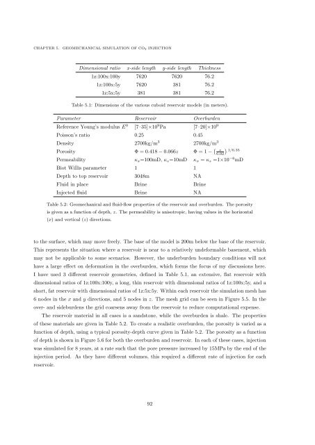
Dimensional ratio x-side length y-side length Thickness
1z:100x:100y 7620 7620 76.2
1z:100x:5y 7620 381 76.2
1z:5x:5y 381 381 76.2
Table 5.1: Dimensions of the various cuboid reservoir models (in meters).
Parameter Reservoir Overburden
Reference Young’s modulus E 0 [7–35]×10 9 Pa [7–20]×10 9
Poisson’s ratio 0.25 0.45
Density 2700kg/m 3 2700kg/m 3
) 1/6.35
Porosity Φ = 0.418 − 0.066z Φ = 1 − ( z
6.02
Permeability κ x =100mD, κ z =10mD κ x = κ z =1×10 −6 mD
Biot Willis parameter 1 1
Depth to top reservoir 3048m NA
Fluid in place Brine Brine
Injected fluid Brine NA
Table 5.2: Geomechanical and fluid-flow properties of the reservoir and overburden. The porosity
is given as a function of depth, z. The permeability is anisotropic, having values in the horizontal
(x) and vertical (z) directions.
to the surface, which may move freely. The base of the model is 200m below the base of the reservoir.
This represents the situation where a reservoir is near to a relatively undeformable basement, which
may not be applicable to some scenarios. However, the underburden boundary conditions will not
have a large effect on deformation in the overburden, which forms the focus of my discussions here.
I have used 3 different reservoir geometries, defined in Table 5.1, an extensive, flat reservoir with
dimensional ratios of 1z:100x:100y, a long, thin reservoir with dimensional ratios of 1z:100x:5y, and a
short, fat reservoir with dimensional ratios of 1z:5x:5y. Within each reservoir the simulation mesh has
6 nodes in the x and y directions, and 5 nodes in z. The mesh grid can be seen in Figure 5.5. In the
over- and sideburdens the grid coarsens away from the reservoir to reduce computational expense.
The reservoir material in all cases is a sandstone, while the overburden is shale. The properties
of these materials are given in Table 5.2. To create a realistic overburden, the porosity is varied as a
function of depth, using a typical porosity-depth curve given in Table 5.2. The porosity as a function
of depth is shown in Figure 5.6 for both the overburden and reservoir. In each of these cases, injection
was simulated for 8 years, at a rate such that the pore pressure increased by 15MPa by the end of the
injection period. As they have different volumes, this required a different rate of injection for each
reservoir.
92