Microseismic Monitoring and Geomechanical Modelling of CO2 - bris

8.3. RESULTS
Marl
Vugg
0.8
0.8
Normalised crack density
0.6
0.4
0.2
Normalised crack density
0.6
0.4
0.2
0
0
−0.2
0 5 10 15 20 25 30
Pressure (MPa)
(a)
−0.2
0 5 10 15 20 25 30
Pressure (MPa)
(b)
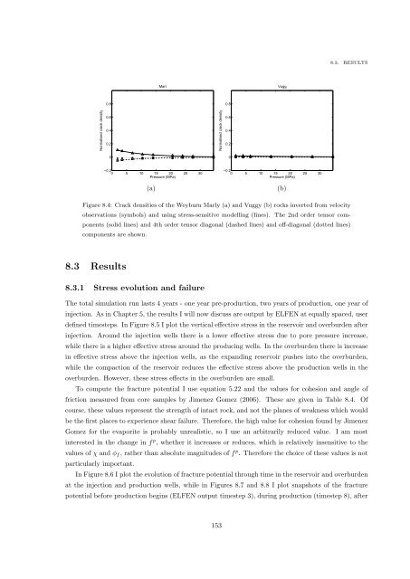
Figure 8.4: Crack densities of the Weyburn Marly (a) and Vuggy (b) rocks inverted from velocity
observations (symbols) and using stress-sensitive modelling (lines). The 2nd order tensor components
(solid lines) and 4th order tensor diagonal (dashed lines) and off-diagonal (dotted lines)
components are shown.
8.3 Results
8.3.1 Stress evolution and failure
The total simulation run lasts 4 years - one year pre-production, two years of production, one year of
injection. As in Chapter 5, the results I will now discuss are output by ELFEN at equally spaced, user
defined timesteps. In Figure 8.5 I plot the vertical effective stress in the reservoir and overburden after
injection. Around the injection wells there is a lower effective stress due to pore pressure increase,
while there is a higher effective stress around the producing wells. In the overburden there is increase
in effective stress above the injection wells, as the expanding reservoir pushes into the overburden,
while the compaction of the reservoir reduces the effective stress above the production wells in the
overburden. However, these stress effects in the overburden are small.
To compute the fracture potential I use equation 5.22 and the values for cohesion and angle of
friction measured from core samples by Jimenez Gomez (2006). These are given in Table 8.4. Of
course, these values represent the strength of intact rock, and not the planes of weakness which would
be the first places to experience shear failure. Therefore, the high value for cohesion found by Jimenez
Gomez for the evaporite is probably unrealistic, so I use an arbitrarily reduced value. I am most
interested in the change in f p , whether it increases or reduces, which is relatively insensitive to the
values of χ and ϕ f , rather than absolute magnitudes of f p . Therefore the choice of these values is not
particularly important.
In Figure 8.6 I plot the evolution of fracture potential through time in the reservoir and overburden
at the injection and production wells, while in Figures 8.7 and 8.8 I plot snapshots of the fracture
potential before production begins (ELFEN output timestep 3), during production (timestep 8), after
153