Microseismic Monitoring and Geomechanical Modelling of CO2 - bris

CHAPTER 4. A COMPARISON OF MICROSEISMIC MONITORING OF FRACTURE STIMULATION DUE TO WATER
VERSUS CO 2 INJECTION
200
150
Recording well
Injection well
2400
2500
Perf shots
Geophones
Northing (m)
100
50
Depth (m)
2600
2700
2800
0
2900
−50
−50 0 50 100 150 200
Easting (m)
(a)
3000
−50 0 50 100 150 200
Easting (m)
(b)
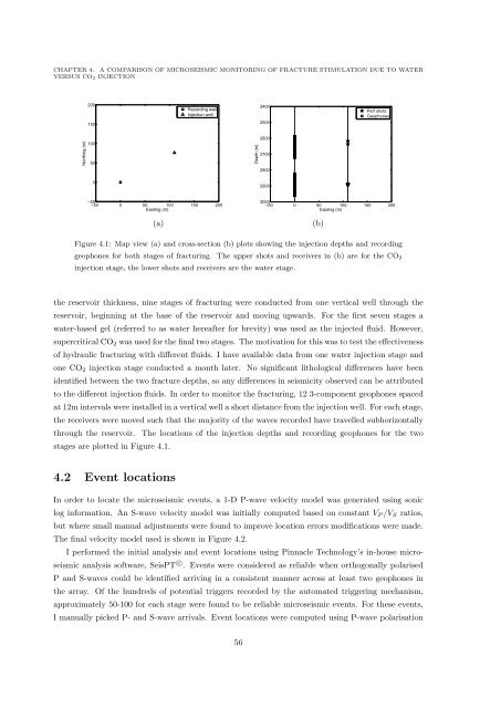
Figure 4.1: Map view (a) and cross-section (b) plots showing the injection depths and recording
geophones for both stages of fracturing. The upper shots and receivers in (b) are for the CO 2
injection stage, the lower shots and receivers are the water stage.
the reservoir thickness, nine stages of fracturing were conducted from one vertical well through the
reservoir, beginning at the base of the reservoir and moving upwards. For the first seven stages a
water-based gel (referred to as water hereafter for brevity) was used as the injected fluid. However,
supercritical CO 2 was used for the final two stages. The motivation for this was to test the effectiveness
of hydraulic fracturing with different fluids. I have available data from one water injection stage and
one CO 2 injection stage conducted a month later. No significant lithological differences have been
identified between the two fracture depths, so any differences in seismicity observed can be attributed
to the different injection fluids. In order to monitor the fracturing, 12 3-component geophones spaced
at 12m intervals were installed in a vertical well a short distance from the injection well. For each stage,
the receivers were moved such that the majority of the waves recorded have travelled subhorizontally
through the reservoir. The locations of the injection depths and recording geophones for the two
stages are plotted in Figure 4.1.
4.2 Event locations
In order to locate the microseismic events, a 1-D P-wave velocity model was generated using sonic
log information. An S-wave velocity model was initially computed based on constant V P /V S ratios,
but where small manual adjustments were found to improve location errors modifications were made.
The final velocity model used is shown in Figure 4.2.
I performed the initial analysis and event locations using Pinnacle Technology’s in-house microseismic
analysis software, SeisPT c⃝ . Events were considered as reliable when orthogonally polarised
P and S-waves could be identified arriving in a consistent manner across at least two geophones in
the array. Of the hundreds of potential triggers recorded by the automated triggering mechanism,
approximately 50-100 for each stage were found to be reliable microseismic events. For these events,
I manually picked P- and S-wave arrivals. Event locations were computed using P-wave polarisation
56