Microseismic Monitoring and Geomechanical Modelling of CO2 - bris

4.2. EVENT LOCATIONS
2400
Velocity Model
P:S velocity ratio
2600
Depth (m)
2800
3000
3200
Sonic log
V P
3400
2000 4000 6000
V S
Velocity (m/s)
0 1
P/S velocity ratio
2
(a)
(b)
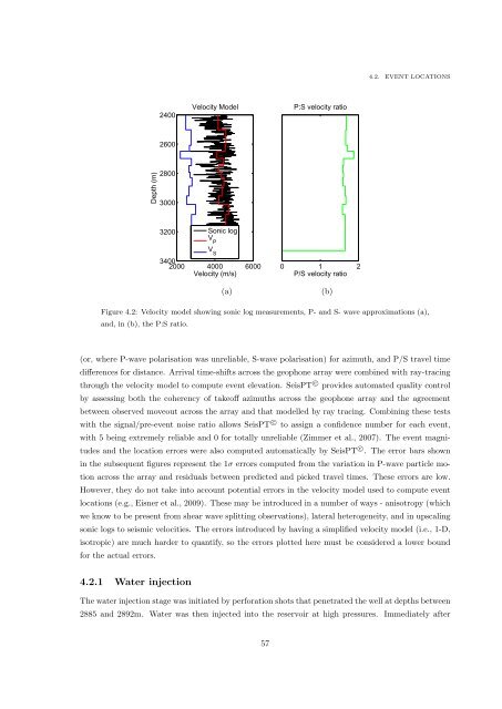
Figure 4.2: Velocity model showing sonic log measurements, P- and S- wave approximations (a),
and, in (b), the P:S ratio.
(or, where P-wave polarisation was unreliable, S-wave polarisation) for azimuth, and P/S travel time
differences for distance. Arrival time-shifts across the geophone array were combined with ray-tracing
through the velocity model to compute event elevation. SeisPT c⃝ provides automated quality control
by assessing both the coherency of takeoff azimuths across the geophone array and the agreement
between observed moveout across the array and that modelled by ray tracing. Combining these tests
with the signal/pre-event noise ratio allows SeisPT c⃝ to assign a confidence number for each event,
with 5 being extremely reliable and 0 for totally unreliable (Zimmer et al., 2007). The event magnitudes
and the location errors were also computed automatically by SeisPT c⃝ . The error bars shown
in the subsequent figures represent the 1σ errors computed from the variation in P-wave particle motion
across the array and residuals between predicted and picked travel times. These errors are low.
However, they do not take into account potential errors in the velocity model used to compute event
locations (e.g., Eisner et al., 2009). These may be introduced in a number of ways - anisotropy (which
we know to be present from shear wave splitting observations), lateral heterogeneity, and in upscaling
sonic logs to seismic velocities. The errors introduced by having a simplified velocity model (i.e., 1-D,
isotropic) are much harder to quantify, so the errors plotted here must be considered a lower bound
for the actual errors.
4.2.1 Water injection
The water injection stage was initiated by perforation shots that penetrated the well at depths between
2885 and 2892m. Water was then injected into the reservoir at high pressures. Immediately after
57