Microseismic Monitoring and Geomechanical Modelling of CO2 - bris

More documents

Recommendations

Info

CHAPTER 3. INVERTING SHEAR-WAVE SPLITTING MEASUREMENTS FOR FRACTURE PROPERTIES Parameter Value Frequency (ω) 100kHz Fluid viscosity (η) 1×10 −3 Pa.s Fracture aperture (c) 2×10 −5 m Fracture aspect ratio (a) 0.0036 Fracture density (ξ) 0.1 Porosity (ϕ) 0.3460 Fluid bulk modulus (K fl ) 2.16GPa Rock shear modulus (µ r ) 12.7GPa Rock bulk modulus (K r ) 16.6GPa P i 50 P ep 3×10 −4 Table 3.1: Physical properties of the synthetic fractured rock created by Rathore et al. (1994), used to test the influence of fractures on ultrasonic velocities. ometry and orientation. These were subsequently dissolved from the matrix using a chemical leachate, leaving the resultant voids to represent a network of fractures whose geometries were known a priori. The seismic velocities of these samples were then measured in the lab at ultrasonic frequencies when both dry and water saturated. Their results provide a benchmark against which the above models can be tested. Table 3.1 lists the relevant parameters for the brine saturated synthetic sandstone constructed by Rathore et al. (1994). Rathore et al. did not compute κ, so I use the estimate given by Hudson et al. (2001) as κ = 300mD. Using these values, P ep ≈ 3 × 10 −4 and P i ≈ 50. Therefore I expect fluid flow to occur and pressure gradients to be fully equalised. As a result, Hudson’s (1981) model, which assumes that fractures are hydraulically isolated, will not be appropriate. Figure 3.3 shows Rathore et al. (1994)’s experimental results along with the modelled values for P- and S-wave velocity assuming isolated fractures in (a) and using frequency dependence in (b). I note in Figure 3.3(a) the P-wave velocity from the experimental results does not match the predictions from Hudson’s 1981 isolated fracture model, of a cos(4ζ) periodicity, where ζ is the incidence angle between the aligned fracture faces and the ultrasonic waves. In contrast, Figure 3.3(b) compares experimental velocities with those predicted from Hudson’s 1996 fluid exchange model, which does account for frequency-dependent flow. It is clear that the fit is far superior, with a cos(2ζ) periodicity. This testing demonstrates the sensitivity of rock physics modelling to the extent of fluid flow, and highlights the need when interpreting data for awareness of the likely extent of fluid flow through estimation of P i and P ep and use of an appropriate model. For seismic waves passing through reservoir rocks, ω is small (10 < ω < 250) and κ is likely to be high. Table 3.2 shows values for the relevant parameters for a generic reservoir example with CO 2 and brine filled fractures, and the resultant values of P ep . It can be seen that P ep for both cases 34
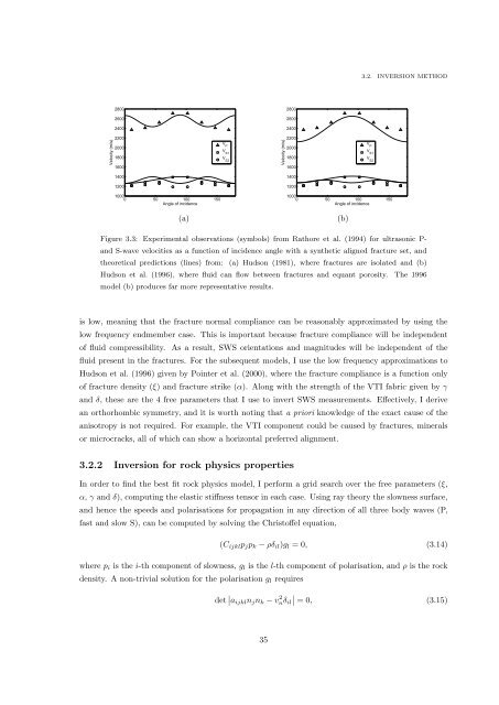
3.2. INVERSION METHOD 2800 2800 2600 2600 2400 2400 Velocity (m/s) 2200 2000 1800 1600 V P V S1 Velocity (m/s) 2200 2000 1800 1600 V S2 0 50 100 150 V P V S1 V S2 1400 1200 1000 0 50 100 150 Angle of incidence (a) 1400 1200 1000 Angle of incidence (b) Figure 3.3: Experimental observations (symbols) from Rathore et al. (1994) for ultrasonic P- and S-wave velocities as a function of incidence angle with a synthetic aligned fracture set, and theoretical predictions (lines) from: (a) Hudson (1981), where fractures are isolated and (b) Hudson et al. (1996), where fluid can flow between fractures and equant porosity. The 1996 model (b) produces far more representative results. is low, meaning that the fracture normal compliance can be reasonably approximated by using the low frequency endmember case. This is important because fracture compliance will be independent of fluid compressibility. As a result, SWS orientations and magnitudes will be independent of the fluid present in the fractures. For the subsequent models, I use the low frequency approximations to Hudson et al. (1996) given by Pointer et al. (2000), where the fracture compliance is a function only of fracture density (ξ) and fracture strike (α). Along with the strength of the VTI fabric given by γ and δ, these are the 4 free parameters that I use to invert SWS measurements. Effectively, I derive an orthorhombic symmetry, and it is worth noting that a priori knowledge of the exact cause of the anisotropy is not required. For example, the VTI component could be caused by fractures, minerals or microcracks, all of which can show a horizontal preferred alignment. 3.2.2 Inversion for rock physics properties In order to find the best fit rock physics model, I perform a grid search over the free parameters (ξ, α, γ and δ), computing the elastic stiffness tensor in each case. Using ray theory the slowness surface, and hence the speeds and polarisations for propagation in any direction of all three body waves (P, fast and slow S), can be computed by solving the Christoffel equation, (C ijkl p j p k − ρδ il )g l = 0, (3.14) where p i is the i-th component of slowness, g l is the l-th component of polarisation, and ρ is the rock density. A non-trivial solution for the polarisation g l requires det ∣ ∣ ∣a ijkl n j n k − vnδ 2 il = 0, (3.15) 35
Page 1: Microseismic Monitoring and Geomech
Page 5 and 6: Abstract Capture of CO 2 produced a
Page 7 and 8: Author’s Declaration I declare th
Page 9 and 10: Acknowledgments There are many thin
Page 11 and 12: Table of Contents Abstract Author
Page 13 and 14: TABLE OF CONTENTS 5.4 Results . . .
Page 15 and 16: Preface ‘Research is not an end i
Page 17 and 18: 6. D. Angus, J-M. Kendall, J.P. Ver
Page 19 and 20: 1 Introduction A technology push ap
Page 21 and 22: 1.2. CCS OVERVIEW Figure 1.2: CCS s
Page 23 and 24: 1.3. THESIS OVERVIEW for CO 2 to be
Page 25 and 26: 1.3. THESIS OVERVIEW as microseismi
Page 27 and 28: 2 The Weyburn CO 2 injection projec
Page 29 and 30: 2.2. WEYBURN GEOLOGICAL SETTING Fig
Page 31 and 32: 2.2. WEYBURN GEOLOGICAL SETTING N F
Page 33 and 34: 2.4. EVENT TIMING AND LOCATIONS 500
Page 35 and 36: 2.4. EVENT TIMING AND LOCATIONS 500
Page 37 and 38: 2.4. EVENT TIMING AND LOCATIONS Nor
Page 39 and 40: 2.4. EVENT TIMING AND LOCATIONS Fig
Page 41 and 42: 2.5. DISCUSSION 500 1000 1100 North
Page 43 and 44: 2.6. SUMMARY 2.6 Summary • CO 2 s
Page 45 and 46: 3 Inverting shear-wave splitting me
Page 47 and 48: 3.2. INVERSION METHOD the additiona
Page 49 and 50: 3.2. INVERSION METHOD 1. P-wave inc
Page 51: 3.2. INVERSION METHOD 180 160 140 C
Page 55 and 56: 3.2. INVERSION METHOD Loop over γ,
Page 57 and 58: 20 10 5 5 1 20 30 40 80 100 60 40 1
Page 59 and 60: 3.4. SWS MEASUREMENTS AT WEYBURN th
Page 61 and 62: 3.4. SWS MEASUREMENTS AT WEYBURN ei
Page 63 and 64: 3.4. SWS MEASUREMENTS AT WEYBURN ξ
Page 65 and 66: 3.4. SWS MEASUREMENTS AT WEYBURN da
Page 67 and 68: 4 2 2 3.4. SWS MEASUREMENTS AT WEYB
Page 69 and 70: 1 1 1 1 1 1 1 1 1 1 3.5. DISCUSSION
Page 71 and 72: 3.6. SUMMARY 3.6 Summary • I have
Page 73 and 74: 4 A comparison of microseismic moni
Page 75 and 76: 4.2. EVENT LOCATIONS 2400 Velocity
Page 77 and 78: 4.2. EVENT LOCATIONS 200 150 Northi
Page 79 and 80: 4.3. EVENT MAGNITUDES Pressure (MPa
Page 81 and 82: 4.3. EVENT MAGNITUDES 160 140 120 N
Page 83 and 84: 4.4. SHEAR WAVE SPLITTING 50 −3 E
Page 85 and 86: 4.5. INITIAL S-WAVE POLARISATION In
Page 87 and 88: 4.5. INITIAL S-WAVE POLARISATION 6
Page 89 and 90: 4.5. INITIAL S-WAVE POLARISATION of
Page 91 and 92: 4.6. INTERPRETATION OF SHEAR WAVE S
Page 93 and 94: 1 1 5 5 30 4.6. INTERPRETATION OF S
Page 95 and 96: 80 4.6. INTERPRETATION OF SHEAR WAV
Page 97 and 98: 2 3 3.5 4 5 2 1.8 1.4 4 4.6. INTERP
Page 99 and 100: 4.7. DISCUSSION 4.7 Discussion The
Page 101 and 102: pressure, P fl σ ′ ij = σ ij
Page 103 and 104:
5.2. EFFECTIVE STRESS AND STRESS PA
Page 105 and 106:
5.3. NUMERICAL MODELLING 5.3.1 Flui
Page 107 and 108:
5.3. NUMERICAL MODELLING MORE FLUID
Page 109 and 110:
5.3. NUMERICAL MODELLING (a) (b) Fi
Page 111 and 112:
5.4. RESULTS 0 500 1000 Depth (m) 1
Page 113 and 114:
5.4. RESULTS 1 0.9 0.8 Soft Med Sti
Page 115 and 116:
5.4. RESULTS Overburden Extension i
Page 117 and 118:
5.4. RESULTS 1z:100x:100y 1z:100x:5
Page 119 and 120:
5.5. SURFACE UPLIFT 1 0.9 0.8 Soft
Page 121 and 122:
5.5. SURFACE UPLIFT Figure 5.17: Ma
Page 123 and 124:
6 Generating anisotropic seismic mo
Page 125 and 126:
6.2. STRESS-SENSITIVE ROCK PHYSICS
Page 127 and 128:
6.3. A MICRO-STRUCTURAL MODEL FOR N
Page 129 and 130:
Page 131 and 132:
Page 133 and 134:
Page 135 and 136:
Page 137 and 138:
Page 139 and 140:
Page 141 and 142:
Page 143 and 144:
Page 145 and 146:
6.4. CALIBRATION WITH LITERATURE DA
Page 147 and 148:
6.4. CALIBRATION WITH LITERATURE DA
Page 149 and 150:
6.5. COMPARISON OF ROCK PHYSICS MOD
Page 151 and 152:
6.5. COMPARISON OF ROCK PHYSICS MOD
Page 153 and 154:
7 Forward modelling of seismic prop
Page 155 and 156:
7.2. SEISMODEL c⃝ WORKFLOW time s
Page 157 and 158:
7.3. RESULTS FROM SIMPLE GEOMECHANI
Page 159 and 160:
Page 161 and 162:
Page 163 and 164:
7.4. SUMMARY 7.4 Summary • I have
Page 165 and 166:
8 Linking geomechanical modelling a
Page 167 and 168:
8.2. MODEL DESCRIPTION Layer Thickn
Page 169 and 170:
8.2. MODEL DESCRIPTION Unit E (GPa)
Page 171 and 172:
8.3. RESULTS Marl Vugg 0.8 0.8 Norm
Page 173 and 174:
8.3. RESULTS 15 10 Injector Produce
Page 175 and 176:
8.3. RESULTS 2000 15 2000 15 1500 1
Page 177 and 178:
8.4. A SOFTER RESERVOIR 8.4 A softe
Page 179 and 180:
8.4. A SOFTER RESERVOIR 2000 15 200
Page 181 and 182:
8.4. A SOFTER RESERVOIR 2000 Max SW
Page 183 and 184:
8.5. DISCUSSION pore-pressure being
Page 185 and 186:
8.6. SUMMARY 8.6 Summary • I appl
Page 187 and 188:
9 Conclusions Geological storage wi
Page 189 and 190:
calibrate. This model has been cali
Page 191 and 192:
9.1. NOVEL CONTRIBUTIONS techniques
Page 193 and 194:
9.2. FUTURE WORK Finally, the compa
Page 195 and 196:
Bibliography Abt, D. L., Fischer, K
Page 197 and 198:
BIBLIOGRAPHY Gassmann, F., 1951. Ub
Page 199 and 200:
BIBLIOGRAPHY Kendall, J.-M., Pilido
Page 201 and 202:
BIBLIOGRAPHY Sayers, C. M., 2002. S
Page 203 and 204:
BIBLIOGRAPHY White, D., 2009. Monit
Page 205 and 206:
A List of Symbols The table below l
Page 207 and 208:
B In Support of Carbon Capture and
Page 209 and 210:
Both China and India are aggressive
Page 211 and 212:
Utsira rock properties vary signifi
show all

Microseismic Monitoring and Geomechanical Modelling of CO2 - bris

You also want an ePaper? Increase the reach of your titles

Delete template?

Save as template?