Microseismic Monitoring and Geomechanical Modelling of CO2 - bris

6.3. A MICRO-STRUCTURAL MODEL FOR NONLINEAR ELASTICITY
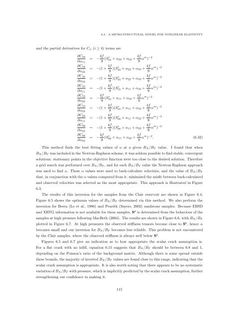
and the partial derivatives for C ii (i ≥ 4) terms are
∂C 44
∂α 11
= − 4f 9 (Sr 44 + α 22 + α 33 + 4f 9 αm ) −2
∂C 44
∂α 22
= −(1 + 4f 9 )(Sr 44 + α 22 + α 33 + 4f 9 αm ) −2
∂C 44
∂α 33
= −(1 + 4f 9 )(Sr 44 + α 22 + α 33 + 4f 9 αm ) −2
∂C 55
∂α 11
= −(1 + 4f 9 )(Sr 55 + α 11 + α 33 + 4f 9 αm ) −2
∂C 55
∂α 22
= − 4f 9 (Sr 55 + α 11 + α 33 + 4f 9 αm ) −2
∂C 55
∂α 33
= −(1 + 4f 9 )(Sr 55 + α 11 + α 33 + 4f 9 αm ) −2
∂C 66
∂α 11
= −(1 + 4f 9 )(Sr 66 + α 11 + α 22 + 4f 9 αm ) −2
∂C 66
∂α 22
= −(1 + 4f 9 )(Sr 66 + α 11 + α 22 + 4f 9 αm ) −2
∂C 66
∂α 33
= − 4f 9 (Sr 66 + α 11 + α 22 + 4f 9 αm ) −2 . (6.32)
This method finds the best fitting values of α at a given B N /B T value. I found that when
B N /B T was included in the Newton-Raphson scheme, it was seldom possible to find stable, convergent
solutions: stationary points in the objective function were too close to the desired solution. Therefore
a grid search was performed over B N /B T , and for each B N /B T value the Newton-Raphson approach
was used to find α. These α values were used to back-calculate velocities, and the value of B N /B T
that, in conjunction with the α values computed from it, minimised the misfit between back-calculated
and observed velocities was selected as the most appropriate. This approach is illustrated in Figure
6.3.
The results of this inversion for the samples from the Clair reservoir are shown in Figure 6.4.
Figure 6.5 shows the optimum values of B N /B T
determined via this method. We also perform the
inversion for Berea (Lo et al., 1986) and Penrith (Sayers, 2002) sandstone samples. Because EBSD
and XRTG information is not available for these samples, S r is determined from the behaviour of the
samples at high pressure following MacBeth (2004). The results are shown in Figure 6.6, with B N /B T
plotted in Figure 6.7. At high pressures the observed stiffness tensors become close to S r , hence α
becomes small and our inversion for B N /B T becomes less reliable. This problem is not encountered
by the Clair samples, where the observed stiffness is always well below S r .
Figures 6.5 and 6.7 give an indication as to how appropriate the scalar crack assumption is.
For a flat crack with no infill, equation 6.15 suggests that B N /B T should be between 0.8 and 1,
depending on the Poisson’s ratio of the background matrix. Although there is some spread outside
these bounds, the majority of inverted B N /B T values are found close to this range, indicating that the
scalar crack assumption is appropriate. It is also worth noting that there appears to be no systematic
variation of B N /B T with pressure, which is implicitly predicted by the scalar crack assumption, further
strengthening our confidence in making it.
115