Microseismic Monitoring and Geomechanical Modelling of CO2 - bris

More documents

Recommendations

Info

CHAPTER 2. THE WEYBURN CO 2 INJECTION PROJECT geochemical analysis and soil gas sampling (Wilson et al., 2004). However, microseismic monitoring was not used at this stage. The 4-D seismic monitoring has been the most successful in imaging CO 2 saturation (White, 2009), where travel time-shifts in the reservoir and reflection amplitude increases at the top of the reservoir are used to image zones of CO 2 saturation (Figure 2.4). In Phase IA the 4-D seismics show the CO 2 plumes migrating out from the horizontal injection wells. In 2003, downhole microseismic monitoring was initiated with a new CO 2 injection site. This stage, named Phase IB and located to the southeast of Phase IA, is the only place at Weyburn so far to use microseismic monitoring. The injection, production and monitoring wells of Phase IB are shown in Figure 2.5. 2.3 Microseismic monitoring at Weyburn Microseismic monitoring seeks to detect the seismic emissions produced by fracturing and fault reactivation around the reservoir. This technique was developed in the early 1990s, and has been used increasingly since then. The magnitudes of such events are such that they cannot usually be detected at the surface, so geophones are placed in boreholes near to the reservoir. When seismic energy is detected at the geophones, event location algorithms are used to locate the source of these emissions, indicating a point in the rock mass that has undergone brittle failure. Seismic energy can also be generated by other subsurface phenomena such as fluid motion through pipes and conduits (e.g., Balmforth et al., 2005), although these processes are not thought to be occurring at Weyburn. It is anticipated that CO 2 injection at Weyburn will alter the pore pressure and stress fields at Weyburn enough to generate failure. By tracking the event locations, the operators hope to track the regions of failure, and thereby the stress changes, and also to assess whether the fracturing presents a risk to the security of storage. 2.3.1 System setup Phase IB has a vertical well (121/06-08) injecting CO 2 at a rate of between 50 - 250 MSCM/day (100-500 tonnes/day). To the northwest and to the southeast are horizontal producing wells (191/11- 08, 192/09-06 and 191/10-08), all running NE-SW. Wells 191/11-08 and 192/09-06 were both in production before the array was installed, while well 191/10-08 was drilled in July 2005, 18 months after CO 2 injection had begun. The injection well was completed in November 2003, with water injection beginning on December 15th. CO 2 injection began on the 21st January. In August 2003 an 8-level, 3-component geophone string was installed in a disused vertical production well (101/06-08) about 50m to the east of the injection well. The sensors were sited at the depths given in Table 2.2. The top of the reservoir in this area is at a depth of 1430m. Surface orientation shots were fired on August 15th, confirming that the geophones had been installed with one component vertical, and the orientations of the horizontal components were calculated from these shots. Apart for some short periods where the system locked up, recording on this system was continuous until November 2004. 14
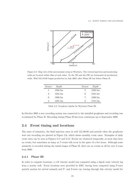
2.4. EVENT TIMING AND LOCATIONS 500 191/11-08 Observation Injector Producer Northing (m) 0 121/06-08 101/06-08 191/10-08 (Jul 2005) 191/09-08 192/09-06 500 500 0 500 Easting (m) Figure 2.5: Map view of the microseismic setup at Weyburn. The vertical injection and monitoring wells are located within 50m of each other. To the NE and the SW are horizontal oil production wells. Well 191/10-08 began production in July 2005, after Phase IB but before Phase II. Sensor Depth Sensor Depth 1 1356.5m 5 1256.5m 2 1331.5m 6 1231.5m 3 1306.5m 7 1206.5m 4 1281.5m 8 1181.5m Table 2.2: Geophone depths for Weyburn Phase IB. In October 2005 a new recording system was connected to the installed geophones and recording was re-initiated for Phase II. Recording during Phase II has been continuous up to September 2009. 2.4 Event timing and locations The rates of seismicity, the fluid injection rates in well 121/06-08 and periods when the geophones were not recording are plotted in Figure 2.6, which shows monthly event rates. Examples of daily event rates can be seen in Figures 2.11 and 2.12. Events are clustered temporally, as most days have no events, but sometimes as many as 7 events will occur in the space of a few hours. Although some seismicity is recorded during the initial stages of Phase II, there are no events at all for over 2 years from 2006. 2.4.1 Phase IB In order to compute locations, a 1-D velocity model was computed using a dipole sonic velocity log from a nearby well. Event locations were provided by ESG, having been computed using P-wave particle motion for arrival azimuth and P- and S-wave ray tracing through this velocity model for 15
Page 1: Microseismic Monitoring and Geomech
Page 5 and 6: Abstract Capture of CO 2 produced a
Page 7 and 8: Author’s Declaration I declare th
Page 9 and 10: Acknowledgments There are many thin
Page 11 and 12: Table of Contents Abstract Author
Page 13 and 14: TABLE OF CONTENTS 5.4 Results . . .
Page 15 and 16: Preface ‘Research is not an end i
Page 17 and 18: 6. D. Angus, J-M. Kendall, J.P. Ver
Page 19 and 20: 1 Introduction A technology push ap
Page 21 and 22: 1.2. CCS OVERVIEW Figure 1.2: CCS s
Page 23 and 24: 1.3. THESIS OVERVIEW for CO 2 to be
Page 25 and 26: 1.3. THESIS OVERVIEW as microseismi
Page 27 and 28: 2 The Weyburn CO 2 injection projec
Page 29 and 30: 2.2. WEYBURN GEOLOGICAL SETTING Fig
Page 31: 2.2. WEYBURN GEOLOGICAL SETTING N F
Page 35 and 36: 2.4. EVENT TIMING AND LOCATIONS 500
Page 37 and 38: 2.4. EVENT TIMING AND LOCATIONS Nor
Page 39 and 40: 2.4. EVENT TIMING AND LOCATIONS Fig
Page 41 and 42: 2.5. DISCUSSION 500 1000 1100 North
Page 43 and 44: 2.6. SUMMARY 2.6 Summary • CO 2 s
Page 45 and 46: 3 Inverting shear-wave splitting me
Page 47 and 48: 3.2. INVERSION METHOD the additiona
Page 49 and 50: 3.2. INVERSION METHOD 1. P-wave inc
Page 51 and 52: 3.2. INVERSION METHOD 180 160 140 C
Page 53 and 54: 3.2. INVERSION METHOD 2800 2800 260
Page 55 and 56: 3.2. INVERSION METHOD Loop over γ,
Page 57 and 58: 20 10 5 5 1 20 30 40 80 100 60 40 1
Page 59 and 60: 3.4. SWS MEASUREMENTS AT WEYBURN th
Page 61 and 62: 3.4. SWS MEASUREMENTS AT WEYBURN ei
Page 63 and 64: 3.4. SWS MEASUREMENTS AT WEYBURN ξ
Page 65 and 66: 3.4. SWS MEASUREMENTS AT WEYBURN da
Page 67 and 68: 4 2 2 3.4. SWS MEASUREMENTS AT WEYB
Page 69 and 70: 1 1 1 1 1 1 1 1 1 1 3.5. DISCUSSION
Page 71 and 72: 3.6. SUMMARY 3.6 Summary • I have
Page 73 and 74: 4 A comparison of microseismic moni
Page 75 and 76: 4.2. EVENT LOCATIONS 2400 Velocity
Page 77 and 78: 4.2. EVENT LOCATIONS 200 150 Northi
Page 79 and 80: 4.3. EVENT MAGNITUDES Pressure (MPa
Page 81 and 82: 4.3. EVENT MAGNITUDES 160 140 120 N
Page 83 and 84:
4.4. SHEAR WAVE SPLITTING 50 −3 E
Page 85 and 86:
4.5. INITIAL S-WAVE POLARISATION In
Page 87 and 88:
4.5. INITIAL S-WAVE POLARISATION 6
Page 89 and 90:
4.5. INITIAL S-WAVE POLARISATION of
Page 91 and 92:
4.6. INTERPRETATION OF SHEAR WAVE S
Page 93 and 94:
1 1 5 5 30 4.6. INTERPRETATION OF S
Page 95 and 96:
80 4.6. INTERPRETATION OF SHEAR WAV
Page 97 and 98:
2 3 3.5 4 5 2 1.8 1.4 4 4.6. INTERP
Page 99 and 100:
4.7. DISCUSSION 4.7 Discussion The
Page 101 and 102:
pressure, P fl σ ′ ij = σ ij
Page 103 and 104:
5.2. EFFECTIVE STRESS AND STRESS PA
Page 105 and 106:
5.3. NUMERICAL MODELLING 5.3.1 Flui
Page 107 and 108:
5.3. NUMERICAL MODELLING MORE FLUID
Page 109 and 110:
5.3. NUMERICAL MODELLING (a) (b) Fi
Page 111 and 112:
5.4. RESULTS 0 500 1000 Depth (m) 1
Page 113 and 114:
5.4. RESULTS 1 0.9 0.8 Soft Med Sti
Page 115 and 116:
5.4. RESULTS Overburden Extension i
Page 117 and 118:
5.4. RESULTS 1z:100x:100y 1z:100x:5
Page 119 and 120:
5.5. SURFACE UPLIFT 1 0.9 0.8 Soft
Page 121 and 122:
5.5. SURFACE UPLIFT Figure 5.17: Ma
Page 123 and 124:
6 Generating anisotropic seismic mo
Page 125 and 126:
6.2. STRESS-SENSITIVE ROCK PHYSICS
Page 127 and 128:
6.3. A MICRO-STRUCTURAL MODEL FOR N
Page 129 and 130:
Page 131 and 132:
Page 133 and 134:
Page 135 and 136:
Page 137 and 138:
Page 139 and 140:
Page 141 and 142:
Page 143 and 144:
Page 145 and 146:
6.4. CALIBRATION WITH LITERATURE DA
Page 147 and 148:
6.4. CALIBRATION WITH LITERATURE DA
Page 149 and 150:
6.5. COMPARISON OF ROCK PHYSICS MOD
Page 151 and 152:
6.5. COMPARISON OF ROCK PHYSICS MOD
Page 153 and 154:
7 Forward modelling of seismic prop
Page 155 and 156:
7.2. SEISMODEL c⃝ WORKFLOW time s
Page 157 and 158:
7.3. RESULTS FROM SIMPLE GEOMECHANI
Page 159 and 160:
Page 161 and 162:
Page 163 and 164:
7.4. SUMMARY 7.4 Summary • I have
Page 165 and 166:
8 Linking geomechanical modelling a
Page 167 and 168:
8.2. MODEL DESCRIPTION Layer Thickn
Page 169 and 170:
8.2. MODEL DESCRIPTION Unit E (GPa)
Page 171 and 172:
8.3. RESULTS Marl Vugg 0.8 0.8 Norm
Page 173 and 174:
8.3. RESULTS 15 10 Injector Produce
Page 175 and 176:
8.3. RESULTS 2000 15 2000 15 1500 1
Page 177 and 178:
8.4. A SOFTER RESERVOIR 8.4 A softe
Page 179 and 180:
8.4. A SOFTER RESERVOIR 2000 15 200
Page 181 and 182:
8.4. A SOFTER RESERVOIR 2000 Max SW
Page 183 and 184:
8.5. DISCUSSION pore-pressure being
Page 185 and 186:
8.6. SUMMARY 8.6 Summary • I appl
Page 187 and 188:
9 Conclusions Geological storage wi
Page 189 and 190:
calibrate. This model has been cali
Page 191 and 192:
9.1. NOVEL CONTRIBUTIONS techniques
Page 193 and 194:
9.2. FUTURE WORK Finally, the compa
Page 195 and 196:
Bibliography Abt, D. L., Fischer, K
Page 197 and 198:
BIBLIOGRAPHY Gassmann, F., 1951. Ub
Page 199 and 200:
BIBLIOGRAPHY Kendall, J.-M., Pilido
Page 201 and 202:
BIBLIOGRAPHY Sayers, C. M., 2002. S
Page 203 and 204:
BIBLIOGRAPHY White, D., 2009. Monit
Page 205 and 206:
A List of Symbols The table below l
Page 207 and 208:
B In Support of Carbon Capture and
Page 209 and 210:
Both China and India are aggressive
Page 211 and 212:
Utsira rock properties vary signifi
show all

Microseismic Monitoring and Geomechanical Modelling of CO2 - bris

You also want an ePaper? Increase the reach of your titles

Delete template?

Save as template?