Microseismic Monitoring and Geomechanical Modelling of CO2 - bris

More documents

Recommendations

Info

CHAPTER 5. GEOMECHANICAL SIMULATION OF CO 2 INJECTION Youngs Modulus (GPa) 0 20 40 60 80 100 0 500 1000 Youngs Modulus (GPa) 0 20 40 60 80 100 0 500 1000 Youngs Modulus (GPa) 0 20 40 60 80 100 0 500 1000 Depth (m) 1500 2000 Overburden Reservoir Depth (m) 1500 2000 Overburden Reservoir Depth (m) 1500 2000 Overburden Reservoir 2500 2500 2500 3000 Ratio 3500 0 1 2 3 4 5 6 Ratio E /E res over 3000 Ratio 3500 0 1 2 3 4 5 6 Ratio E /E res over 3000 Ratio 3500 0 1 2 3 4 5 6 Ratio E /E res over (a) (b) (c) 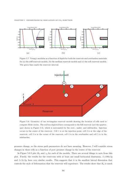Figure 5.7: Young’s modulus as a function of depth for both the reservoir and overburden materials for (a) the stiff reservoir models, (b) the medium reservoir models and (c) the soft reservoir models. The green lines mark the reservoir interval. Injection well 4 2 3 z y 1 5 x Reservoir Figure 5.8: Geometry of our rectangular reservoir models showing the location of cells used to compute Mohr circles. The red box depicted here corresponds to the full reservoir (not the quarterspot shown in Figure 5.5), which is surrounded by the over-, under- and sideburden. Injection occurs in the centre of the reservoir. Cell 1 is at the injection point, cell 2 is at the edge of the reservoir, cell 3 is in the corner of the reservoir, cell 4 is in the overburden and cell 5 is in the sideburden. pressure change, so the stress path parameters do not have meaning. However, I will consider stress changes in these cells as a function of pore pressure change in the centre of the reservoir. In Figure 5.9 I plot K 0 and γ 3 for each of the models. There are several things to note from this plot. Firstly, the results for the reservoirs with at least one small horizontal dimension, 1z:100x:5y and 1z:5x:5y, have very similar results. This suggests that it is the smallest lateral dimension that controls the style of deformation that the reservoir will experience. The results show that K 0 is much 94
5.4. RESULTS 1 0.9 0.8 Soft Med Stiff 1 0.9 0.8 1 0.9 0.8 1 0.9 0.8 0.7 0.7 0.7 0.7 0.6 0.6 0.6 0.6 K 0 0.5 γ 3 0.5 K 0 0.5 γ 3 0.5 0.4 0.4 0.4 0.4 0.3 0.3 0.3 0.3 0.2 0.2 0.2 0.2 0.1 0.1 0.1 0.1 0 1 2 3 0 1 2 3 0 1 2 3 0 1 2 3 (a) 1 1 (b) 0.9 0.9 0.8 0.8 0.7 0.7 0.6 0.6 K 0 0.5 γ 3 0.5 0.4 0.4 0.3 0.3 0.2 0.2 0.1 0.1 0 1 2 3 0 1 2 3 (c) Figure 5.9: Numerical results for stress path parameters as a function of reservoir geometry and stiffness. The flat, extensive reservoir (1z:100x:100y) is shown in (a), the long thin reservoir (1z:100x:5y) is in (b) and the short, fat reservoir (1z:5x:5y) is in (c). There are 3 models for each geometry, with a soft, medium and stiff reservoir. I plot K 0 in the left hand panels and γ 3 in the right hand panels, for the cells at the centre (1), edge (2) and corner (3) of the reservoir. larger for the smaller reservoirs. It is also slightly larger for elevated reservoir:overburden stiffness ratios, and for cells at the edge of the reservoir (cells 2 and 3). K 0 describes the change in size of the Mohr circle, with a low value of K 0 meaning a reduction in size. Given that a large Mohr circle is more likely to cross the failure envelope, this suggests that small, stiff reservoirs are more likely to fail, and that this effect is most significant at the edges of the reservoir. The implications that this has for rock failure and microseismic activity will discussed below. I find that γ 3 is largest for low reservoir:overburden stiffness ratios, and small for elevated reservoir:overburden stiffness ratios. It is larger at the edges of the reservoirs, and larger for the small reservoirs. γ 3 can be interpreted as a stress arching indicator - a small γ 3 implies that the applied stress does not change during injection, so the change in effective stress is controlled entirely by the change in pore pressure, and therefore is hydrostatic. 95
Page 1:
Microseismic Monitoring and Geomech
Page 5 and 6:
Abstract Capture of CO 2 produced a
Page 7 and 8:
Author’s Declaration I declare th
Page 9 and 10:
Acknowledgments There are many thin
Page 11 and 12:
Table of Contents Abstract Author
Page 13 and 14:
TABLE OF CONTENTS 5.4 Results . . .
Page 15 and 16:
Preface ‘Research is not an end i
Page 17 and 18:
6. D. Angus, J-M. Kendall, J.P. Ver
Page 19 and 20:
1 Introduction A technology push ap
Page 21 and 22:
1.2. CCS OVERVIEW Figure 1.2: CCS s
Page 23 and 24:
1.3. THESIS OVERVIEW for CO 2 to be
Page 25 and 26:
1.3. THESIS OVERVIEW as microseismi
Page 27 and 28:
2 The Weyburn CO 2 injection projec
Page 29 and 30:
2.2. WEYBURN GEOLOGICAL SETTING Fig
Page 31 and 32:
2.2. WEYBURN GEOLOGICAL SETTING N F
Page 33 and 34:
2.4. EVENT TIMING AND LOCATIONS 500
Page 35 and 36:
2.4. EVENT TIMING AND LOCATIONS 500
Page 37 and 38:
2.4. EVENT TIMING AND LOCATIONS Nor
Page 39 and 40:
2.4. EVENT TIMING AND LOCATIONS Fig
Page 41 and 42:
2.5. DISCUSSION 500 1000 1100 North
Page 43 and 44:
2.6. SUMMARY 2.6 Summary • CO 2 s
Page 45 and 46:
3 Inverting shear-wave splitting me
Page 47 and 48:
3.2. INVERSION METHOD the additiona
Page 49 and 50:
3.2. INVERSION METHOD 1. P-wave inc
Page 51 and 52:
3.2. INVERSION METHOD 180 160 140 C
Page 53 and 54:
3.2. INVERSION METHOD 2800 2800 260
Page 55 and 56:
3.2. INVERSION METHOD Loop over γ,
Page 57 and 58:
20 10 5 5 1 20 30 40 80 100 60 40 1
Page 59 and 60:
3.4. SWS MEASUREMENTS AT WEYBURN th
Page 61 and 62: 3.4. SWS MEASUREMENTS AT WEYBURN ei
Page 63 and 64: 3.4. SWS MEASUREMENTS AT WEYBURN ξ
Page 65 and 66: 3.4. SWS MEASUREMENTS AT WEYBURN da
Page 67 and 68: 4 2 2 3.4. SWS MEASUREMENTS AT WEYB
Page 69 and 70: 1 1 1 1 1 1 1 1 1 1 3.5. DISCUSSION
Page 71 and 72: 3.6. SUMMARY 3.6 Summary • I have
Page 73 and 74: 4 A comparison of microseismic moni
Page 75 and 76: 4.2. EVENT LOCATIONS 2400 Velocity
Page 77 and 78: 4.2. EVENT LOCATIONS 200 150 Northi
Page 79 and 80: 4.3. EVENT MAGNITUDES Pressure (MPa
Page 81 and 82: 4.3. EVENT MAGNITUDES 160 140 120 N
Page 83 and 84: 4.4. SHEAR WAVE SPLITTING 50 −3 E
Page 85 and 86: 4.5. INITIAL S-WAVE POLARISATION In
Page 87 and 88: 4.5. INITIAL S-WAVE POLARISATION 6
Page 89 and 90: 4.5. INITIAL S-WAVE POLARISATION of
Page 91 and 92: 4.6. INTERPRETATION OF SHEAR WAVE S
Page 93 and 94: 1 1 5 5 30 4.6. INTERPRETATION OF S
Page 95 and 96: 80 4.6. INTERPRETATION OF SHEAR WAV
Page 97 and 98: 2 3 3.5 4 5 2 1.8 1.4 4 4.6. INTERP
Page 99 and 100: 4.7. DISCUSSION 4.7 Discussion The
Page 101 and 102: pressure, P fl σ ′ ij = σ ij
Page 103 and 104: 5.2. EFFECTIVE STRESS AND STRESS PA
Page 105 and 106: 5.3. NUMERICAL MODELLING 5.3.1 Flui
Page 107 and 108: 5.3. NUMERICAL MODELLING MORE FLUID
Page 109 and 110: 5.3. NUMERICAL MODELLING (a) (b) Fi
Page 111: 5.4. RESULTS 0 500 1000 Depth (m) 1
Page 115 and 116: 5.4. RESULTS Overburden Extension i
Page 117 and 118: 5.4. RESULTS 1z:100x:100y 1z:100x:5
Page 119 and 120: 5.5. SURFACE UPLIFT 1 0.9 0.8 Soft
Page 121 and 122: 5.5. SURFACE UPLIFT Figure 5.17: Ma
Page 123 and 124: 6 Generating anisotropic seismic mo
Page 125 and 126: 6.2. STRESS-SENSITIVE ROCK PHYSICS
Page 127 and 128: 6.3. A MICRO-STRUCTURAL MODEL FOR N
Page 145 and 146: 6.4. CALIBRATION WITH LITERATURE DA
Page 147 and 148: 6.4. CALIBRATION WITH LITERATURE DA
Page 149 and 150: 6.5. COMPARISON OF ROCK PHYSICS MOD
Page 151 and 152: 6.5. COMPARISON OF ROCK PHYSICS MOD
Page 153 and 154: 7 Forward modelling of seismic prop
Page 155 and 156: 7.2. SEISMODEL c⃝ WORKFLOW time s
Page 157 and 158: 7.3. RESULTS FROM SIMPLE GEOMECHANI
Page 163 and 164:
7.4. SUMMARY 7.4 Summary • I have
Page 165 and 166:
8 Linking geomechanical modelling a
Page 167 and 168:
8.2. MODEL DESCRIPTION Layer Thickn
Page 169 and 170:
8.2. MODEL DESCRIPTION Unit E (GPa)
Page 171 and 172:
8.3. RESULTS Marl Vugg 0.8 0.8 Norm
Page 173 and 174:
8.3. RESULTS 15 10 Injector Produce
Page 175 and 176:
8.3. RESULTS 2000 15 2000 15 1500 1
Page 177 and 178:
8.4. A SOFTER RESERVOIR 8.4 A softe
Page 179 and 180:
8.4. A SOFTER RESERVOIR 2000 15 200
Page 181 and 182:
8.4. A SOFTER RESERVOIR 2000 Max SW
Page 183 and 184:
8.5. DISCUSSION pore-pressure being
Page 185 and 186:
8.6. SUMMARY 8.6 Summary • I appl
Page 187 and 188:
9 Conclusions Geological storage wi
Page 189 and 190:
calibrate. This model has been cali
Page 191 and 192:
9.1. NOVEL CONTRIBUTIONS techniques
Page 193 and 194:
9.2. FUTURE WORK Finally, the compa
Page 195 and 196:
Bibliography Abt, D. L., Fischer, K
Page 197 and 198:
BIBLIOGRAPHY Gassmann, F., 1951. Ub
Page 199 and 200:
BIBLIOGRAPHY Kendall, J.-M., Pilido
Page 201 and 202:
BIBLIOGRAPHY Sayers, C. M., 2002. S
Page 203 and 204:
BIBLIOGRAPHY White, D., 2009. Monit
Page 205 and 206:
A List of Symbols The table below l
Page 207 and 208:
B In Support of Carbon Capture and
Page 209 and 210:
Both China and India are aggressive
Page 211 and 212:
Utsira rock properties vary signifi
show all

Microseismic Monitoring and Geomechanical Modelling of CO2 - bris

You also want an ePaper? Increase the reach of your titles

Delete template?

Save as template?