Microseismic Monitoring and Geomechanical Modelling of CO2 - bris

8.2. MODEL DESCRIPTION
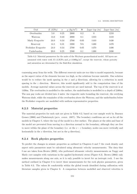
Unit E (GPa) ν ρ (kg/m 3 ) Φ Layer top (m) Layer base (m)
Overburden 5.0 0.25 2000 0.2 0 1210
Watrous 14.0 0.23 2000 0.1 1210 1410
Marly Evaporite 24.0 0.34 2700 0.05 1410 1430
Reservoir 14.5 0.31 2200 NA 1430 1470
Frobisher Evaporite 24.0 0.34 2700 0.05 1470 1490
Underburden 20.0 0.25 2500 0.1 1490 2490
Table 8.2: Material parameters for the units of the Weyburn geomechanical model. All layers are
saturated with water with K=2.2GPa and ρ=1100kg/m 3 , except the reservoir, whose porosity
and saturation are determined by the fluid-flow simulation.
coarsening away from the wells. The different reservoir units are too thin to model separately, because
as the aspect ratios of the elements become too high, so the solutions become unstable. One solution
would be to reduce the mesh spacing in the x and y directions, allowing for a reduction in mesh
spacing in the z direction. However, this would significantly add to the computation time of the
models. Average material values across the reservoir are used instead. The top of the reservoir is at
1430m. The overburden is modelled to the surface, the underburden is modelled to a depth of 2480m.
The non pay rocks are divided into 4 units: the evaporite units bounding the reservoir, the overlying
Watrous shale, while the remainder of the overburden above the Watrous, and the underburden below
the Frobisher evaporite are modelled with uniform representative properties.
8.2.3 Material properties
The material properties for each unit are given in Table 8.2, based on core sample work by Jimenez
Gomez (2006) and Chalaturnyk (pers. comm. 2007 ). The boundary conditions are set as for all the
models in Chapter 5, where the top of the model is a free surface. The planes at the sides and base of
the model are prevented from moving in a direction normal to the boundary, although they are free
to move within the plane of the boundary (i.e. at the x − z boundary, nodes can move vertically and
horizontally in the x direction, but not in the y direction).
8.2.4 Rock physics properties
To predict the changes in seismic properties as outlined in Chapters 6 and 7 the crack density and
aspect ratio parameters must be calculated using ultrasonic velocity measurements. The data that
I use are taken from Brown (2002), who performed ultrasonic velocity measurements on Vuggy and
Marly core samples with variations in the applied hydrostatic stress (Figure 8.3). Brown (2002) only
makes measurements along one axis, so it is only possible to invert for an isotropic rock. I use the
method outlined in Chapter 6 to invert these measurements for the rock physics parameters, given
in Table 8.3. The values fit comfortably within the global trends identified during calibration with
literature samples given in Chapter 6. A comparison between modelled and observed velocities is
151