Microseismic Monitoring and Geomechanical Modelling of CO2 - bris

4
2
2
3.4. SWS MEASUREMENTS AT WEYBURN
270°
300°
240°
330°
210°
0°
180°
30°
150°
60°
120°
Anisotropy [%]
21
20
19
18
17
16
15
14
13
12
11
10
9
8
7
6
5
4
3
2
1
0
90°
(a)
Frac density 2
0.3
0.25
0.2
0.15
0.1
0.05
1.5
1
1.5
1
2
1.5
0
0 0.05 0.1 0.15 0.2 0.25 0.3
Frac density 1
(b)
1
1.5
2
1
Frac strike 2
180
160
140
120
100
80
60
40
20
2
3
2
1
3
3
4
1.5
1
1.5
5
4
0
0 50 100 150
Frac strike 1
1.5
6
2
1
2
3
5
(c)
4
1
3
1.5
6
5
2
6
4
2
1.5
1
5
1.5
3
3
2
4
4
1.5
2
3
2
2
180
160
2
3
5
4
180
160
1.5
1
1.5
140
6
140
1.5
1
Frac strike 1
120
100
80
60
40
20
1.5
1.5
2
1
3
2
1.5
2
1
1
0
0 0.05 0.1 0.15 0.2 0.25 0.3
Frac density 1
1.5
1.5
(d)
2 2
3
3
4
5
1
1.5
Frac strike 2
120
100
80
60
40
20
2
2
0
0 0.05 0.1 0.15 0.2 0.25 0.3
Frac density 2
(e)
2
3
2
3
1.5
2
3
4
4
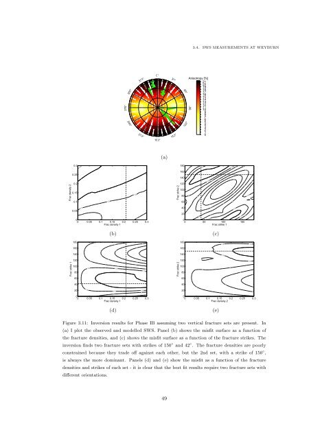
Figure 3.11: Inversion results for Phase IB assuming two vertical fracture sets are present. In
(a) I plot the observed and modelled SWS. Panel (b) shows the misfit surface as a function of
the fracture densities, and (c) shows the misfit surface as a function of the fracture strikes. The
inversion finds two fracture sets with strikes of 150 ◦ and 42 ◦ . The fracture densities are poorly
constrained because they trade off against each other, but the 2nd set, with a strike of 150 ◦ ,
is always the more dominant. Panels (d) and (e) show the misfit as a function of the fracture
densities and strikes of each set - it is clear that the best fit results require two fracture sets with
different orientations.
49