Microseismic Monitoring and Geomechanical Modelling of CO2 - bris

5.4. RESULTS
1z:100x:100y 1z:100x:5y 1z:5x:5y
10
10
10
5
5
5
Soft
∆ f p
0
−5
∆ f p
0
−5
∆ f p
0
−5
−10
−10
−10
−15
1 2 3 4 5 6
Timestep
−15
1 2 3 4 5 6
Timestep
−15
1 2 3 4 5 6
Timestep
10
10
10
5
5
5
Medium
∆ f p
0
−5
∆ f p
0
−5
∆ f p
0
−5
−10
−10
−10
−15
1 2 3 4 5 6
Timestep
−15
1 2 3 4 5 6
Timestep
−15
1 2 3 4 5 6
Timestep
10
10
10
5
5
5
Stiff
∆ f p
0
−5
∆ f p
0
−5
∆ f p
0
−5
−10
−10
−10
−15
1 2 3 4 5 6
Timestep
−15
1 1.5 2 2.5 3 3.5 4 4.5 5
Timestep
−15
1 2 3 4 5 6
Timestep
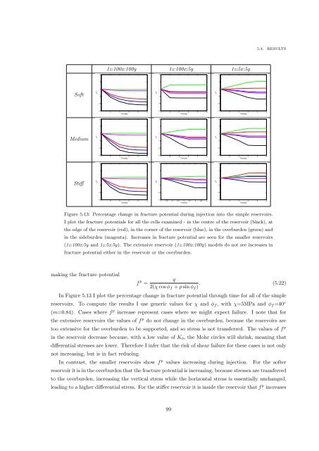
Figure 5.13: Percentage change in fracture potential during injection into the simple reservoirs.
I plot the fracture potentials for all the cells examined - in the centre of the reservoir (black), at
the edge of the reservoir (red), in the corner of the reservoir (blue), in the overburden (green) and
in the sideburden (magenta). Increases in fracture potential are seen for the smaller reservoirs
(1z:100x:5y and 1z:5x:5y). The extensive reservoir (1z:100x:100y) models do not see increases in
fracture potential either in the reservoir or the overburden.
making the fracture potential
f p =
q
2(χ cos ϕ f + p sin ϕ f ) . (5.22)
In Figure 5.13 I plot the percentage change in fracture potential through time for all of the simple
reservoirs.
To compute the results I use generic values for χ and ϕ f , with χ=5MPa and ϕ f =40 ◦
(m=0.84). Cases where f p increase represent cases where we might expect failure. I note that for
the extensive reservoirs the values of f p do not change in the overburden, because the reservoirs are
too extensive for the overburden to be supported, and so stress is not transferred. The values of f p
in the reservoir decrease because, with a low value of K 0 , the Mohr circles will shrink, meaning that
differential stresses are lower. Therefore I infer that the risk of shear failure for these cases is not only
not increasing, but is in fact reducing.
In contrast, the smaller reservoirs show f p values increasing during injection. For the softer
reservoir it is in the overburden that the fracture potential is increasing, because stresses are transferred
to the overburden, increasing the vertical stress while the horizontal stress is essentially unchanged,
leading to a higher differential stress. For the stiffer reservoir it is inside the reservoir that f p increases
99