Microseismic Monitoring and Geomechanical Modelling of CO2 - bris

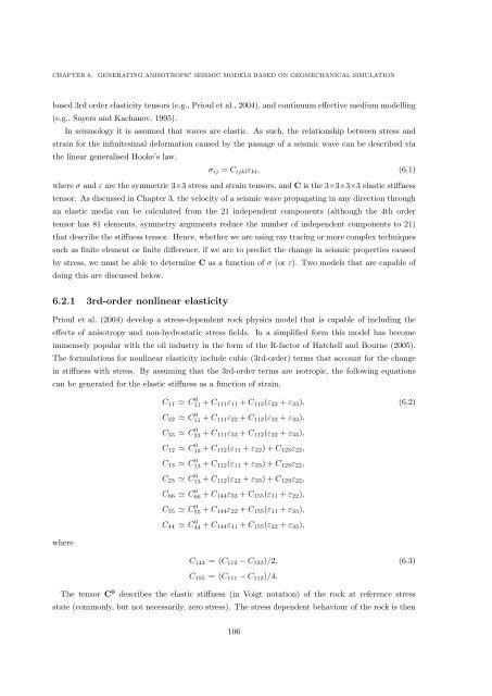
CHAPTER 6.
GENERATING ANISOTROPIC SEISMIC MODELS BASED ON GEOMECHANICAL SIMULATION
based 3rd order elasticity tensors (e.g., Prioul et al., 2004), and continuum effective medium modelling
(e.g., Sayers and Kachanov, 1995).
In seismology it is assumed that waves are elastic. As such, the relationship between stress and
strain for the infinitesimal deformation caused by the passage of a seismic wave can be described via
the linear generalised Hooke’s law,
σ ij = C ijkl ε kl , (6.1)
where σ and ε are the symmetric 3×3 stress and strain tensors, and C is the 3×3×3×3 elastic stiffness
tensor. As discussed in Chapter 3, the velocity of a seismic wave propagating in any direction through
an elastic media can be calculated from the 21 independent components (although the 4th order
tensor has 81 elements, symmetry arguments reduce the number of independent components to 21)
that describe the stiffness tensor. Hence, whether we are using ray tracing or more complex techniques
such as finite element or finite difference, if we are to predict the change in seismic properties caused
by stress, we must be able to determine C as a function of σ (or ε). Two models that are capable of
doing this are discussed below.
6.2.1 3rd-order nonlinear elasticity
Prioul et al. (2004) develop a stress-dependent rock physics model that is capable of including the
effects of anisotropy and non-hydrostatic stress fields. In a simplified form this model has become
immensely popular with the oil industry in the form of the R-factor of Hatchell and Bourne (2005).
The formulations for nonlinear elasticity include cubic (3rd-order) terms that account for the change
in stiffness with stress. By assuming that the 3rd-order terms are isotropic, the following equations
can be generated for the elastic stiffness as a function of strain,
C 11 ≃ C11 0 + C 111 ε 11 + C 112 (ε 22 + ε 33 ), (6.2)
C 22 ≃ C11 0 + C 111 ε 22 + C 112 (ε 22 + ε 33 ),
C 33 ≃ C33 0 + C 111 ε 33 + C 112 (ε 22 + ε 33 ),
C 12 ≃ C12 0 + C 112 (ε 11 + ε 22 ) + C 123 ε 22 ,
C 13 ≃ C13 0 + C 112 (ε 11 + ε 33 ) + C 123 ε 22 ,
C 23 ≃ C13 0 + C 112 (ε 22 + ε 33 ) + C 123 ε 22 ,
C 66 ≃ C66 0 + C 144 ε 33 + C 155 (ε 11 + ε 22 ),
C 55 ≃ C55 0 + C 144 ε 22 + C 155 (ε 11 + ε 33 ),
C 44 ≃ C44 0 + C 144 ε 11 + C 155 (ε 22 + ε 33 ),
where
C 144 = (C 112 − C 123 )/2, (6.3)
C 155 = (C 111 − C 112 )/4.
The tensor C 0 describes the elastic stiffness (in Voigt notation) of the rock at reference stress
state (commonly, but not necessarily, zero stress). The stress dependent behaviour of the rock is then
106