Microseismic Monitoring and Geomechanical Modelling of CO2 - bris

4.5. INITIAL S-WAVE POLARISATION
6
10
9
8
7
6
5
4
3
2
1
0
0 20 40 60 80 100 120 140 160 180
S polarisation (degrees from vertical)
(a)
5
4
3
2
1
0
0 20 40 60 80 100 120 140 160 180
S polarisation (degrees from vertical)
(b)
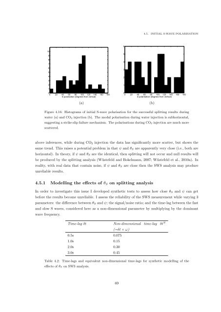
Figure 4.16: Histograms of initial S-wave polarisation for the successful splitting results during
water (a) and CO 2 injection (b). The modal polarisation during water injection is subhorizontal,
suggesting a strike-slip failure mechanism. The polarisations during CO 2 injection are much more
scattered.
above inferences, while during CO 2 injection the data has significantly more scatter, but shows the
same trend. This raises a potential problem in that ψ and θ S are apparently very close (i.e., both are
horizontal). In theory, if ψ and θ S are the identical, then splitting will not occur and null results will
be produced by the splitting analysis (Wüstefeld and Bokelmann, 2007; Wüstefeld et al., 2010a). In
reality, with real data that contain noise, if ψ and θ S are close then the SWS analysis may produce
unreliable results.
4.5.1 Modelling the effects of θ S on splitting analysis
In order to investigate this issue I developed synthetic tests to assess how close θ S and ψ can get
before the results become unreliable. I assess the reliability of the SWS measurement while varying 3
parameters: the difference between θ S and ψ; the signal/noise ratio; and the time-lag between the fast
and slow S waves, considered here as a non-dimensional parameter by multiplying by the dominant
wave frequency.
Time-lag δt Non-dimensional time-lag δt N
(=δt × ω)
0.5s 0.075
1.0s 0.15
2.0s 0.30
3.0s 0.45
Table 4.2: Time-lags and equivalent non-dimensional time-lags for synthetic modelling of the
effects of θ S on SWS analysis.
69