Microseismic Monitoring and Geomechanical Modelling of CO2 - bris

20
10
5
5
1
20
30
40
80
100
60
40
1
20
80
3.3. SYNTHETIC TESTING OF INVERSION METHOD
330°
0°
30°
Anisotropy [%]
5
300°
60°
4
3
270°
90°
2
240°
120°
1
210°
180°
150°
0
(a)
0.2
0.2
30
100
γ
0.18
0.16
0.14
0.12
0.1
0.08
200
200
100
60
80
200
δ
0.18
0.16
0.14
0.12
0.1
0.08
100
60
80 80
40
30
20
10
5
10
5
20
10
30
40
60
80
100
0.06
0.04
0.02
100
100
80
60
40
0
0 20 40 60 80 100 120 140 160 180
Fracture Strike (α)
30
10
5
20
20
30
40
40
60
100
80
0.06
0.04
0.02
100
100
0
0 20 40 60 80 100 120 140 160 180
Fracture Strike (α)
20
30
40
60
(b)
0.2
(c)
0.18
0.16
80
40
30
40
80
100
30
20
200 200
0.14
0.12
60
10
60
δ
0.1
0.08
40
30
0.06
10
0.04
60
60
0.02
100
80
20
0
0 0.05 0.1 0.15 0.2
γ
(d)
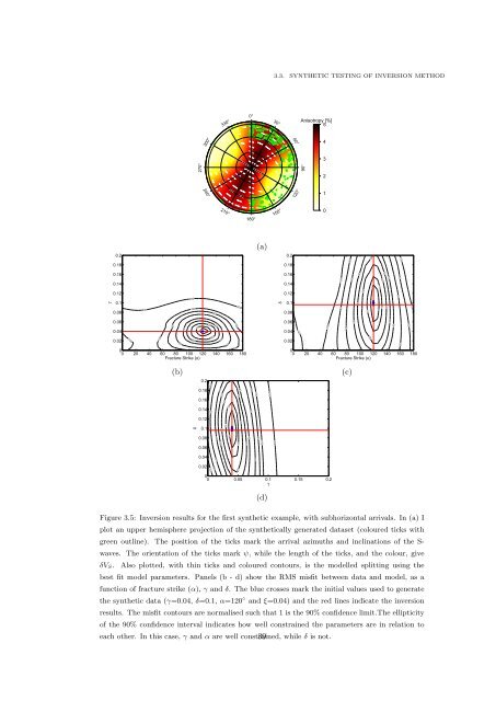
Figure 3.5: Inversion results for the first synthetic example, with subhorizontal arrivals. In (a) I
plot an upper hemisphere projection of the synthetically generated dataset (coloured ticks with
green outline). The position of the ticks mark the arrival azimuths and inclinations of the S-
waves. The orientation of the ticks mark ψ, while the length of the ticks, and the colour, give
δV S.
Also plotted, with thin ticks and coloured contours, is the modelled splitting using the
best fit model parameters. Panels (b - d) show the RMS misfit between data and model, as a
function of fracture strike (α), γ and δ. The blue crosses mark the initial values used to generate
the synthetic data (γ=0.04, δ=0.1, α=120 ◦ and ξ=0.04) and the red lines indicate the inversion
results. The misfit contours are normalised such that 1 is the 90% confidence limit.The ellipticity
of the 90% confidence interval indicates how well constrained the parameters are in relation to
each other. In this case, γ and α are well constrained, 39 while δ is not.