Microseismic Monitoring and Geomechanical Modelling of CO2 - bris

8.2. MODEL DESCRIPTION
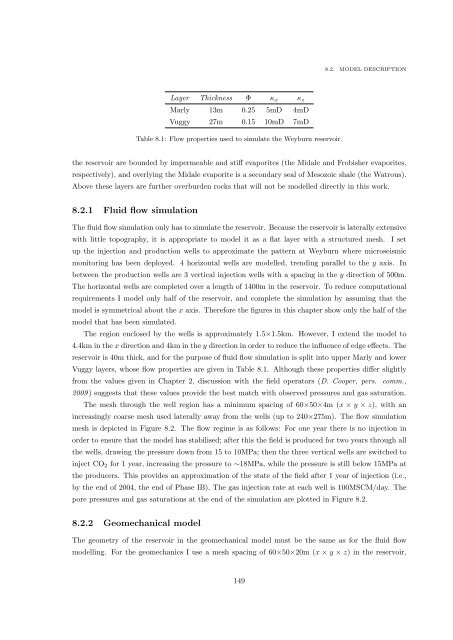
Layer Thickness Φ κ x κ z
Marly 13m 0.25 5mD 4mD
Vuggy 27m 0.15 10mD 7mD
Table 8.1: Flow properties used to simulate the Weyburn reservoir.
the reservoir are bounded by impermeable and stiff evaporites (the Midale and Frobisher evaporites,
respectively), and overlying the Midale evaporite is a secondary seal of Mesozoic shale (the Watrous).
Above these layers are further overburden rocks that will not be modelled directly in this work.
8.2.1 Fluid flow simulation
The fluid flow simulation only has to simulate the reservoir. Because the reservoir is laterally extensive
with little topography, it is appropriate to model it as a flat layer with a structured mesh. I set
up the injection and production wells to approximate the pattern at Weyburn where microseismic
monitoring has been deployed. 4 horizontal wells are modelled, trending parallel to the y axis. In
between the production wells are 3 vertical injection wells with a spacing in the y direction of 500m.
The horizontal wells are completed over a length of 1400m in the reservoir. To reduce computational
requirements I model only half of the reservoir, and complete the simulation by assuming that the
model is symmetrical about the x axis. Therefore the figures in this chapter show only the half of the
model that has been simulated.
The region enclosed by the wells is approximately 1.5×1.5km. However, I extend the model to
4.4km in the x direction and 4km in the y direction in order to reduce the influence of edge effects. The
reservoir is 40m thick, and for the purpose of fluid flow simulation is split into upper Marly and lower
Vuggy layers, whose flow properties are given in Table 8.1. Although these properties differ slightly
from the values given in Chapter 2, discussion with the field operators (D. Cooper, pers. comm.,
2009 ) suggests that these values provide the best match with observed pressures and gas saturation.
The mesh through the well region has a minimum spacing of 60×50×4m (x × y × z), with an
increasingly coarse mesh used laterally away from the wells (up to 240×275m). The flow simulation
mesh is depicted in Figure 8.2. The flow regime is as follows: For one year there is no injection in
order to ensure that the model has stabilised; after this the field is produced for two years through all
the wells, drawing the pressure down from 15 to 10MPa; then the three vertical wells are switched to
inject CO 2 for 1 year, increasing the pressure to ∼18MPa, while the pressure is still below 15MPa at
the producers. This provides an approximation of the state of the field after 1 year of injection (i.e.,
by the end of 2004, the end of Phase IB). The gas injection rate at each well is 100MSCM/day. The
pore pressures and gas saturations at the end of the simulation are plotted in Figure 8.2.
8.2.2 Geomechanical model
The geometry of the reservoir in the geomechanical model must be the same as for the fluid flow
modelling. For the geomechanics I use a mesh spacing of 60×50×20m (x × y × z) in the reservoir,
149