Microseismic Monitoring and Geomechanical Modelling of CO2 - bris

7.2. SEISMODEL c⃝ WORKFLOW
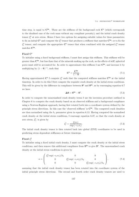
time step, is equal to C in . These are the stiffness of the background rock C r (which corresponds
to the idealised case of the rock mass without any compliant porosity); and the initial crack density
tensor ξi
0 at zero stress. Hence I have two options for assigning suitable values for these parameters:
to fix an initial C r and compute the ξi 0 tensor that produces a stiffness that matches Cin ; or to fix the
ξ 0 i tensor, and compute the appropriate C r tensor that when combined with the assigned ξ 0 i tensor
matches C in .
Fixed C r
To initialise using a fixed background stiffness, I must first assign this stiffness. This stiffness will be
greater than C in , but less than that of the minerals making up the rock, as the effects of stiff, spherical
pores must still be accounted for. In order to approximate this stiffness I use C in , and increase it by
multiplying by (1 − Φ) −1 , such that
C r =
Cin
1 − Φ . (7.1)
Having approximated C r I compute ξi
0 such that the computed stiffness matches C in at the initial
timestep. In order to do this I first compute the requisite crack density at the initial stress conditions.
This will be given by the difference in compliance between S r and S in , as by rearranging equation 6.7
we have
∆S = S in − S r . (7.2)
In order to compute the unnormalised crack density terms I use the inversion procedure outlined in
Chapter 6 to compute the crack density based on an observed stiffness and a background compliance
using a Newton-Raphson approach, having first rotated both into a coordinate system defined by the
principle stress directions. In this case the ‘observed stiffness’ is C in . The computed crack densities
are then normalised using the h i parameter given in equation 6.13. Having computed the normalised
crack density at the initial stress conditions, I rearrange equation 6.37, so that the crack density at
zero stress, ξ 0 i , is given by ξ 0 i =
ξ(σ i )
exp (−c r σ i ) . (7.3)
The initial crack density tensor is then rotated back into global (ENZ) coordinates to be used in
predicting stress dependent stiffnesses at future timesteps.
Fixed ξ 0 i
To initialise using a fixed initial crack density, I must compute the crack density at the initial stress
conditions, and then remove this additional compliance from S in to give S r . The unnormalised crack
density at the initial stress conditions is given by
⎛
⎞
0 0
ξ1 0 exp(−c r σ 1 )/h 1 0 0
α = ⎜
⎝ 0 ξ2 0 exp(−c r σ 2 )/h 2 0 ⎟
⎠ , (7.4)
assuming that the initial crack density tensor has been rotated into the coordinate system of the
initial principle stress directions.
The second and fourth order crack density tensors are used to
137