Microseismic Monitoring and Geomechanical Modelling of CO2 - bris

CHAPTER 4. A COMPARISON OF MICROSEISMIC MONITORING OF FRACTURE STIMULATION DUE TO WATER
VERSUS CO 2 INJECTION
3
3
0.25
2.5
0.25
2.5
(Signal:Noise) −1
0.2
0.15
0.1
2
1.5
1
(Signal:Noise) −1
0.2
0.15
0.1
2
1.5
1
0.05
0.5
0.05
0.5
0
0 5 10 15 20
θ S
−ψ
25 30 35
0
0
0 5 10 15 20
θ S
−ψ
25 30 35
0
(a)
(b)
3
3
0.25
2.5
0.25
2.5
(Signal:Noise) −1
0.2
0.15
0.1
2
1.5
1
(Signal:Noise) −1
0.2
0.15
0.1
2
1.5
1
0.05
0.5
0.05
0.5
0
0 5 10 15 20
θ −ψ S
25 30 35
0
0
0 5 10 15 20
θ −ψ S
25 30 35
0
(c)
(d)
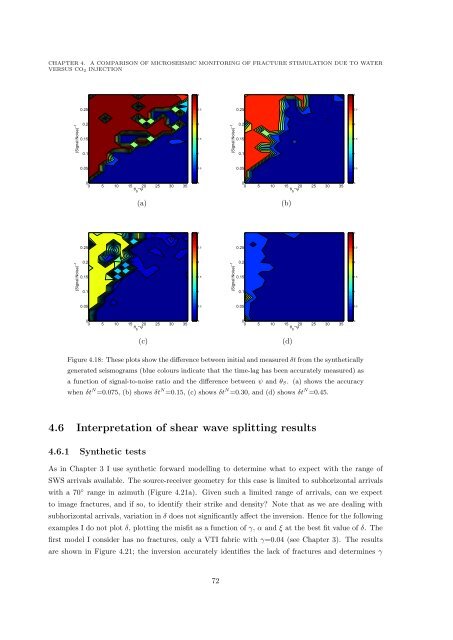
Figure 4.18: These plots show the difference between initial and measured δt from the synthetically
generated seismograms (blue colours indicate that the time-lag has been accurately measured) as
a function of signal-to-noise ratio and the difference between ψ and θ S . (a) shows the accuracy
when δt N =0.075, (b) shows δt N =0.15, (c) shows δt N =0.30, and (d) shows δt N =0.45.
4.6 Interpretation of shear wave splitting results
4.6.1 Synthetic tests
As in Chapter 3 I use synthetic forward modelling to determine what to expect with the range of
SWS arrivals available. The source-receiver geometry for this case is limited to subhorizontal arrivals
with a 70 ◦ range in azimuth (Figure 4.21a). Given such a limited range of arrivals, can we expect
to image fractures, and if so, to identify their strike and density Note that as we are dealing with
subhorizontal arrivals, variation in δ does not significantly affect the inversion. Hence for the following
examples I do not plot δ, plotting the misfit as a function of γ, α and ξ at the best fit value of δ. The
first model I consider has no fractures, only a VTI fabric with γ=0.04 (see Chapter 3). The results
are shown in Figure 4.21; the inversion accurately identifies the lack of fractures and determines γ
72