

Microseismic Monitoring and Geomechanical Modelling of CO2 - bris
Microseismic Monitoring and Geomechanical Modelling of CO2 - bris
Microseismic Monitoring and Geomechanical Modelling of CO2 - bris

Create successful ePaper yourself
Turn your PDF publications into a flip-book with our unique Google optimized e-Paper software.
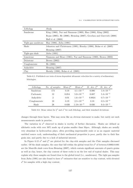
6.4. CALIBRATION WITH LITERATURE DATA<br />
Lithology<br />
Study<br />
S<strong>and</strong>stone King (1966), Nur <strong>and</strong> Simmons (1969), Han (1986), King (2002)<br />
Rojas (2005), He (2006), Hemsing (2007), Grochau <strong>and</strong> Gurevich (2008)<br />
Hall et al. (2008)<br />
Tight-gas s<strong>and</strong>stone Han (1986), Jizba (1991)<br />
Shale Johnston <strong>and</strong> Christensen (1995), Hornby (1998), Bolas et al. (2005)<br />
Hemsing (2007)<br />
Tight-gas shale Jizba (1991)<br />
Limestone Simmons <strong>and</strong> Brace (1965), Nur <strong>and</strong> Simmons (1969), Brown (2002)<br />
Dolostone Brown (2002)<br />
Conglomerate He (2006)<br />
Anhydrite Hemsing (2007)<br />
Clay Hornby (1998), Bolas et al. (2005)<br />
Table 6.5: Published core tests <strong>of</strong> stress dependent ultrasonic velocities for a variety <strong>of</strong> sedimentary<br />
lithologies.<br />
Lithology No. <strong>of</strong> samples Mean ξ 0 Mean a 0 St. dev. ξ 0 St. dev. a 0<br />
S<strong>and</strong>stone 174 0.10 4.1×10 −4 0.080 1.8×10 −4<br />
Carbonate 12 0.054 5.9×10 −4 0.087 5.4×10 −4<br />
Anhydrite 2 0.01 1.6×10 −4 0.0024 0.7×10 −4<br />
Conglomerate 10 0.19 2.5×10 −4 0.18 0.5×10 −4<br />
Shale 26 0.026 1.18×10 −3 0.026 9.4×10 −4<br />
Table 6.6: Mean values for ξ 0 <strong>and</strong> a 0 for each lithology, <strong>and</strong> their st<strong>and</strong>ard deviations.<br />
changes through these layers. This may seem like an obvious statement to make, but rarely are such<br />
measurements made in practise.<br />
The variation in a 0 observed in shales is worthy <strong>of</strong> further discussion. Shales are defined as<br />
siliclastic rocks with over 50% made up <strong>of</strong> grains smaller than 50µm. Although, shales are usually<br />
very abundant in hydrocarbon plays, <strong>of</strong>ten providing impermeable seals or as an organic material<br />
enriched source rock, underst<strong>and</strong>ing <strong>of</strong> their mechanical properties is poor, partly due to their fine<br />
grain size, <strong>and</strong> partly due to a lack <strong>of</strong> industrial interest.<br />
In Figure 6.12 a 0 <strong>and</strong> ξ 0 are plotted for the clay-rich samples <strong>and</strong> the Clair samples discussed<br />
earlier. Of the shale samples, the ones that fall within the global trend for a 0 <strong>of</strong> between 0.0002-0.001<br />
are the Manville shale cores from Hemsing (2007), which contain significant amounts <strong>of</strong> quartz grains<br />
as well as clay, hence, the clay content <strong>of</strong> these rocks is on the low end <strong>of</strong> typical shales. This may<br />
explain why these samples are found close to the global trend (i.e., s<strong>and</strong>stones). The tight gas samples<br />
from Jizba (1991) are also found to have a 0 estimates that are sensitive to clay content, with elevated<br />
a 0 for samples with a high clay content.<br />
127


