Microseismic Monitoring and Geomechanical Modelling of CO2 - bris

5.4. RESULTS
1
0.9
0.8
Soft
Med
Stiff
1
0.9
0.8
1
0.9
0.8
1
0.9
0.8
0.7
0.7
0.7
0.7
0.6
0.6
0.6
0.6
K 0
0.5
γ 3
0.5
K 0
0.5
γ 3
0.5
0.4
0.4
0.4
0.4
0.3
0.3
0.3
0.3
0.2
0.2
0.2
0.2
0.1
0.1
0.1
0.1
0
1 2 3
0
1 2 3
0
1 2 3
0
1 2 3
(a)
1
1
(b)
0.9
0.9
0.8
0.8
0.7
0.7
0.6
0.6
K 0
0.5
γ 3
0.5
0.4
0.4
0.3
0.3
0.2
0.2
0.1
0.1
0
1 2 3
0
1 2 3
(c)
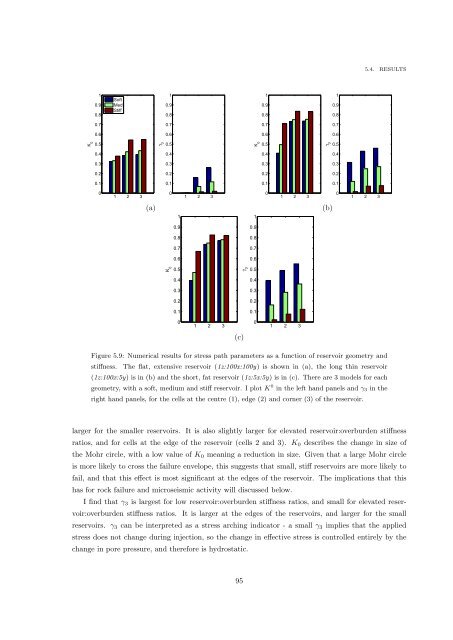
Figure 5.9: Numerical results for stress path parameters as a function of reservoir geometry and
stiffness. The flat, extensive reservoir (1z:100x:100y) is shown in (a), the long thin reservoir
(1z:100x:5y) is in (b) and the short, fat reservoir (1z:5x:5y) is in (c). There are 3 models for each
geometry, with a soft, medium and stiff reservoir. I plot K 0 in the left hand panels and γ 3 in the
right hand panels, for the cells at the centre (1), edge (2) and corner (3) of the reservoir.
larger for the smaller reservoirs. It is also slightly larger for elevated reservoir:overburden stiffness
ratios, and for cells at the edge of the reservoir (cells 2 and 3). K 0 describes the change in size of
the Mohr circle, with a low value of K 0 meaning a reduction in size. Given that a large Mohr circle
is more likely to cross the failure envelope, this suggests that small, stiff reservoirs are more likely to
fail, and that this effect is most significant at the edges of the reservoir. The implications that this
has for rock failure and microseismic activity will discussed below.
I find that γ 3 is largest for low reservoir:overburden stiffness ratios, and small for elevated reservoir:overburden
stiffness ratios. It is larger at the edges of the reservoirs, and larger for the small
reservoirs. γ 3 can be interpreted as a stress arching indicator - a small γ 3 implies that the applied
stress does not change during injection, so the change in effective stress is controlled entirely by the
change in pore pressure, and therefore is hydrostatic.
95