Microseismic Monitoring and Geomechanical Modelling of CO2 - bris

CHAPTER 3.
INVERTING SHEAR-WAVE SPLITTING MEASUREMENTS FOR FRACTURE PROPERTIES
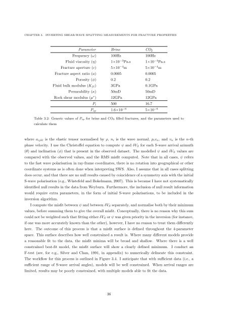
Parameter Brine CO 2
Frequency (ω) 100Hz 100Hz
Fluid viscosity (η) 1×10 −3 Pa.s 1×10 −4 Pa.s
Fracture aperture (c) 5×10 −4 m 5×10 −4 m
Fracture aspect ratio (a) 0.0005 0.0005
Porosity (ϕ) 0.2 0.2
Fluid bulk modulus (K fl ) 3GPa 0.1GPa
Permeability (κ) 50mD 50mD
Rock shear modulus (µ r ) 12GPa 12GPa
P i 500 16.7
P ep 1.6×10 −6 5×10 −6
Table 3.2: Generic values of P ep for brine and CO 2 filled fractures, and the parameters used to
calculate them
where a ijkl is the elastic tensor normalised by ρ, n i is the wave normal, p i v n , and v n is the n-th
phase velocity. I use the Christoffel equation to compute ψ and δV S for each S-wave arrival azimuth
(θ) and inclination (ϕ) that is present in the observed dataset. The modelled ψ and δV S values are
compared with the observed values, and the RMS misfit computed. Note that in all cases, ψ refers
to the fast wave polarisation in ray-frame coordinates, there is no rotation into geographical or other
coordinate systems as is often done when interpreting SWS. Also, I assume that in all cases splitting
does occur, and that there are no null results caused by coincidence of a symmetry axis with the initial
S-wave polarisation (e.g., Wüstefeld and Bokelmann, 2007). This is because I have not systematically
identified null results in the data from Weyburn. Furthermore, the inclusion of null result information
would require extra parameters, in the form of initial S-wave polarisations, to be included in the
inversion algorithm.
I compute the misfit between ψ and between δV S separately, and normalise both by their minimum
values, before summing them to give the overall misfit. Conceptually, there is no reason why this sum
could not be weighted such that fitting either δV S or ψ was given priority in the inversion (for instance,
if one was more accurately known than the other), however, I have no reason to treat them differently
here. The outcome of this process is that a misfit surface is defined throughout the 4-parameter
space. This surface describes how well constrained a result is. Where many different models provide
a reasonable fit to the data, the misfit minima will be broad and shallow. Where there is a well
constrained best-fit model, the misfit surface will show a clearly defined minimum. I conduct an
F-test (see, for e.g., Silver and Chan, 1991, in appendix) to numerically delineate this constraint.
The workflow for this process is outlined in Figure 3.4. I anticipate that with sufficient data (i.e., a
sufficient range of S-wave arrival angles), models will be well constrained. When arrival ranges are
limited, results may be poorly constrained, with multiple models able to fit the data.
36