

Microseismic Monitoring and Geomechanical Modelling of CO2 - bris
Microseismic Monitoring and Geomechanical Modelling of CO2 - bris
Microseismic Monitoring and Geomechanical Modelling of CO2 - bris

Create successful ePaper yourself
Turn your PDF publications into a flip-book with our unique Google optimized e-Paper software.
3.2. INVERSION METHOD<br />
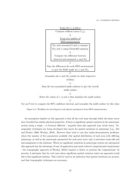
Loop over γ, ξ <strong>and</strong> α<br />
Compute stiffness tensor C ijkl<br />
⇓<br />
Loop over number <strong>of</strong><br />
SWS measurements<br />
For each measured θ <strong>and</strong> ϕ compute<br />
δV S <strong>and</strong> ψ using Christ<strong>of</strong>fel equation<br />
⇓<br />
Compute the difference between<br />
observed <strong>and</strong> measured ψ <strong>and</strong> δV S<br />
⇓<br />
Sum the differences for each SWS measurement<br />
to give the RMS misfit for ψ <strong>and</strong> δV S<br />
⇓<br />
Normalise the ψ <strong>and</strong> δV S misfits by their respective<br />
minima<br />
⇓<br />
Sum the two normalised misfit surfaces to give the overall<br />
misfit surface<br />
⇓<br />
Select the values <strong>of</strong> γ, ξ <strong>and</strong> α that minimise the misfit surface<br />
⇓<br />
Use an F-test to compute the 90% confidence interval, <strong>and</strong> normalise the misfit surface by this value<br />
Figure 3.4: Workflow for inverting for rock physics parameters from SWS measurements.<br />
An assumption implicit in this approach is that all the rock mass through which the shear waves<br />
have travelled has similar physical properties. If there is significant spatial variation in the anisotropic<br />
system along a single - or between different - raypaths then this approach may break down. Tomographic<br />
techniques are being developed that invert for spatial variations in anisotropy (e.g., Abt<br />
<strong>and</strong> Fischer, 2008; Wookey, 2010). However these tend to run into under-determination problems,<br />
where the number <strong>of</strong> free parameters available (the spatial distribution <strong>of</strong> each area with differing<br />
anisotropy, as well as the anisotropic parameters for each area) serve only to introduce trade-<strong>of</strong>fs <strong>and</strong><br />
non-uniqueness to the solutions. Where no significant variations in anisotropic system are anticipated<br />
this approach has the advantage <strong>of</strong> ease <strong>of</strong> application <strong>and</strong> much reduced computational requirements<br />
- the tomographic approach <strong>of</strong> Wookey (2010) requires a cluster to perform the computations! In<br />
practise, I anticipate that for real cases where significant spatial variation exists our approach would<br />
fail to find significant minima. This could be used as an indication that spatial variations are present,<br />
<strong>and</strong> that tomographic techniques are necessary.<br />
37


