Microseismic Monitoring and Geomechanical Modelling of CO2 - bris

4.6. INTERPRETATION OF SHEAR WAVE SPLITTING RESULTS
6
6
5
5
4
4
3
3
2
2
1
1
0
−150 −100 −50 0 50 100 150
ψ − θ S
(degrees)
0
−150 −100 −50 0 50 100 150
ψ − θ S
(degrees)
(a)
(b)
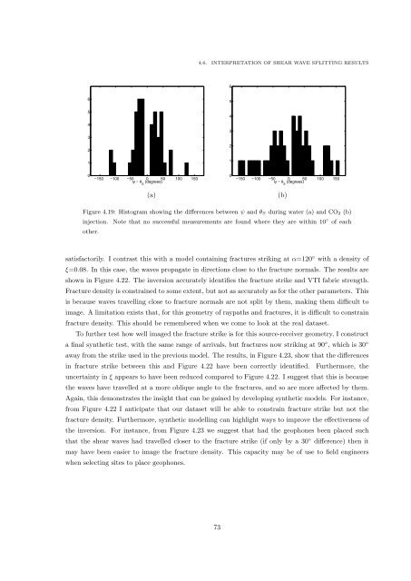
Figure 4.19: Histogram showing the differences between ψ and θ S during water (a) and CO 2 (b)
injection. Note that no successful measurements are found where they are within 10 ◦ of each
other.
satisfactorily. I contrast this with a model containing fractures striking at α=120 ◦ with a density of
ξ=0.08. In this case, the waves propagate in directions close to the fracture normals. The results are
shown in Figure 4.22. The inversion accurately identifies the fracture strike and VTI fabric strength.
Fracture density is constrained to some extent, but not as accurately as for the other parameters. This
is because waves travelling close to fracture normals are not split by them, making them difficult to
image. A limitation exists that, for this geometry of raypaths and fractures, it is difficult to constrain
fracture density. This should be remembered when we come to look at the real dataset.
To further test how well imaged the fracture strike is for this source-receiver geometry, I construct
a final synthetic test, with the same range of arrivals, but fractures now striking at 90 ◦ , which is 30 ◦
away from the strike used in the previous model. The results, in Figure 4.23, show that the differences
in fracture strike between this and Figure 4.22 have been correctly identified. Furthermore, the
uncertainty in ξ appears to have been reduced compared to Figure 4.22. I suggest that this is because
the waves have travelled at a more oblique angle to the fractures, and so are more affected by them.
Again, this demonstrates the insight that can be gained by developing synthetic models. For instance,
from Figure 4.22 I anticipate that our dataset will be able to constrain fracture strike but not the
fracture density. Furthermore, synthetic modelling can highlight ways to improve the effectiveness of
the inversion. For instance, from Figure 4.23 we suggest that had the geophones been placed such
that the shear waves had travelled closer to the fracture strike (if only by a 30 ◦ difference) then it
may have been easier to image the fracture density. This capacity may be of use to field engineers
when selecting sites to place geophones.
73