entropia di entanglement in teorie invarianti conformi bidimensionali

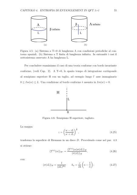
CAPITOLO 4. ENTROPIA DI ENTANGLEMENT IN QFT 1+1 55
Λ
L
(a)
β infinito
L
Λ
β infinito
Figura 4.5: (a) Sistema a T=0 di lunghezza Λ con condizioni periodiche al contorno
spaziali. (b) Sistema a T finita di lunghezza infinita. In entrambi i casi il
sottosistema osservato A ha lunghezza L.
Per concludere esaminiamo il caso di una teoria conforme con bordo invariante
conforme, (vedi Cap. 2). A T=0, lo spazio tempo di integrazione corrisponde
al semipiano superiore H con un taglio, ad esempio lungo l’ asse immaginario
0 ≤ Im(w) ≤ L. Una condizione al bordo conforme è assunta in Im(w) = 0.
La mappa:
H
L
0
(b)
Figura 4.6: Semipiano H superiore, tagliato.
z =
1
w − iL n
, (4.25)
w + iL
trasforma la superficie di Riemann in un disco D. Procedendo come nel par. 4.3
si ottiene:
con:
〈T (n) (w)〉Rn = 〈T (n) (w)σ(iL)〉H
, (4.26)
〈σ(iL)〉H
〈σ(iL)〉H =
1
(2L) 2hσ
hσ = c
n −
24
1
; (4.27)
n