Nichtlineare Methoden zur Quantifizierung von Abhängigkeiten und ...

18 KAPITEL 2. GRUNDLAGEN DER INFORMATIONSTHEORIE
(c)
0 1 0 1 1 0 0 X i
c
0 1 0 1 0 1 0 Y i
i−3
i−2
i−1
i i+1 i+2 i+3
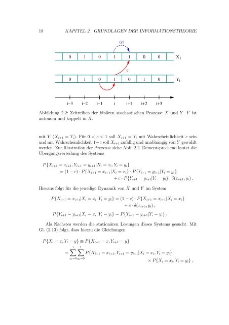
Abbildung 2.2: Zeitreihen der binären stochastischen Prozesse X und Y . Y ist
autonom und koppelt in X.
mit Y (X i+1 = Y i ). Für 0 < c < 1 soll X i+1 = Y i mit Wahrscheinlichkeit c sein
und mit Wahrscheinlichkeit 1−c soll X i+1 zufällig und unabhängig von Y gewählt
werden. Zur Illustration der Prozesse siehe Abb. 2.2. Dementsprechend lautet die
Übergangsverteilung des Systems
P {X i+1 = x i+1 , Y i+1 = y i+1 |X i = x i , Y i = y i }
= (1 − c) · P {X i+1 = x i+1 |X i = x i } · P {Y i+1 = y i+1 |Y i = y i }
+ c · P {Y i+1 = y i+1 |Y i = y i } · δ(x i+1 , y i ) .
Hieraus folgt für die jeweilige Dynamik von X und Y im System
P {X i+1 = x i+1 |X i = x i , Y i = y i } = (1 − c) · P {X i+1 = x i+1 |X i = x i }
+ c · δ(x i+1 , y i ) ,
P {Y i+1 = y i+1 |X i = x i , Y i = y i } = P {Y i+1 = y i+1 |Y i = y i } .
Als Nächstes werden die stationären Lösungen dieses Systems gesucht. Mit
Gl. (2.13) folgt, dass hierzu die Gleichungen
P {X i = x, Y i = y} ≡ P {X i+1 = x, Y i+1 = y}
1∑ 1∑
= P {X i+1 = x i+1 , Y i+1 = y i+1 |X i = x i , Y i = y i }
x i =0 y i =0
× P {X i = x i , Y i = y i } ,